autobinning
Perform automatic binning of given predictors
Description
sc = autobinning(sc)
Automatic binning finds binning maps or rules to bin numeric data and to group
categories of categorical data. The binning rules are stored in the
creditscorecard object. To apply the binning rules to the
creditscorecard object data, or to a new dataset, use
bindata.
sc = autobinning(sc,PredictorNames)PredictorNames.
Automatic binning finds binning maps or rules to bin numeric data and to group
categories of categorical data. The binning rules are stored in the
creditscorecard object. To apply the binning rules to the
creditscorecard object data, or to a new dataset, use
bindata.
sc = autobinning(___,Name,Value)PredictorNames using optional name-value pair
arguments. See the name-value argument Algorithm for a
description of the supported binning algorithms.
Automatic binning finds binning maps or rules to bin numeric data and to group
categories of categorical data. The binning rules are stored in the
creditscorecard object. To apply the binning rules to the
creditscorecard object data, or to a new dataset, use
bindata.
Examples
Create a creditscorecard object using the CreditCardData.mat file to load the data (using a dataset from Refaat 2011).
load CreditCardData
sc = creditscorecard(data,'IDVar','CustID');
Perform automatic binning using the default options. By default, autobinning bins all predictors and uses the Monotone algorithm.
sc = autobinning(sc);
Use bininfo to display the binned data for the predictor CustAge.
bi = bininfo(sc, 'CustAge')bi=8×6 table
Bin Good Bad Odds WOE InfoValue
_____________ ____ ___ ______ _________ _________
{'[-Inf,33)'} 70 53 1.3208 -0.42622 0.019746
{'[33,37)' } 64 47 1.3617 -0.39568 0.015308
{'[37,40)' } 73 47 1.5532 -0.26411 0.0072573
{'[40,46)' } 174 94 1.8511 -0.088658 0.001781
{'[46,48)' } 61 25 2.44 0.18758 0.0024372
{'[48,58)' } 263 105 2.5048 0.21378 0.013476
{'[58,Inf]' } 98 26 3.7692 0.62245 0.0352
{'Totals' } 803 397 2.0227 NaN 0.095205
Use plotbins to display the histogram and WOE curve for the predictor CustAge.
plotbins(sc,'CustAge')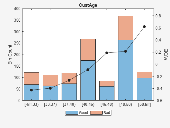
Create a creditscorecard object using the CreditCardData.mat file to load the data (using a dataset from Refaat 2011).
load CreditCardData
sc = creditscorecard(data);
Perform automatic binning for the predictor CustIncome using the default options. By default, autobinning uses the Monotone algorithm.
sc = autobinning(sc,'CustIncome');Use bininfo to display the binned data.
bi = bininfo(sc, 'CustIncome')bi=8×6 table
Bin Good Bad Odds WOE InfoValue
_________________ ____ ___ _______ _________ __________
{'[-Inf,29000)' } 53 58 0.91379 -0.79457 0.06364
{'[29000,33000)'} 74 49 1.5102 -0.29217 0.0091366
{'[33000,35000)'} 68 36 1.8889 -0.06843 0.00041042
{'[35000,40000)'} 193 98 1.9694 -0.026696 0.00017359
{'[40000,42000)'} 68 34 2 -0.011271 1.0819e-05
{'[42000,47000)'} 164 66 2.4848 0.20579 0.0078175
{'[47000,Inf]' } 183 56 3.2679 0.47972 0.041657
{'Totals' } 803 397 2.0227 NaN 0.12285
Create a creditscorecard object using the CreditCardData.mat file to load the data (using a dataset from Refaat 2011).
load CreditCardData
sc = creditscorecard(data);
Perform automatic binning for the predictor CustIncome using the Monotone algorithm with the initial number of bins set to 20. This example explicitly sets both the Algorithm and the AlgorithmOptions name-value arguments.
AlgoOptions = {'InitialNumBins',20};
sc = autobinning(sc,'CustIncome','Algorithm','Monotone','AlgorithmOptions',...
     AlgoOptions);
Use bininfo to display the binned data. Here, the cut points, which delimit the bins, are also displayed.
[bi,cp] = bininfo(sc,'CustIncome')bi=11×6 table
Bin Good Bad Odds WOE InfoValue
_________________ ____ ___ _______ _________ __________
{'[-Inf,19000)' } 2 3 0.66667 -1.1099 0.0056227
{'[19000,29000)'} 51 55 0.92727 -0.77993 0.058516
{'[29000,31000)'} 29 26 1.1154 -0.59522 0.017486
{'[31000,34000)'} 80 42 1.9048 -0.060061 0.0003704
{'[34000,35000)'} 33 17 1.9412 -0.041124 7.095e-05
{'[35000,40000)'} 193 98 1.9694 -0.026696 0.00017359
{'[40000,42000)'} 68 34 2 -0.011271 1.0819e-05
{'[42000,43000)'} 39 16 2.4375 0.18655 0.001542
{'[43000,47000)'} 125 50 2.5 0.21187 0.0062972
{'[47000,Inf]' } 183 56 3.2679 0.47972 0.041657
{'Totals' } 803 397 2.0227 NaN 0.13175
cp = 9×1

       19000
       29000
       31000
       34000
       35000
       40000
       42000
       43000
       47000
This example shows how to use the autobinning default Monotone algorithm and the AlgorithmOptions name-value pair arguments associated with the Monotone algorithm. The AlgorithmOptions for the Monotone algorithm are three name-value pair parameters: ‘InitialNumBins', 'Trend', and 'SortCategories'. 'InitialNumBins' and 'Trend' are applicable for numeric predictors and 'Trend' and 'SortCategories' are applicable for categorical predictors.
Create a creditscorecard object using the CreditCardData.mat file to load the data (using a dataset from Refaat 2011).
load CreditCardData
sc = creditscorecard(data,'IDVar','CustID');
Perform automatic binning for the numeric predictor CustIncome using the Monotone algorithm with 20 bins. This example explicitly sets both the Algorithm argument and the AlgorithmOptions name-value arguments for 'InitialNumBins' and 'Trend'.
AlgoOptions = {'InitialNumBins',20,'Trend','Increasing'};

sc = autobinning(sc,'CustIncome','Algorithm','Monotone',...
    'AlgorithmOptions',AlgoOptions);
Use bininfo to display the binned data.
bi = bininfo(sc,'CustIncome')bi=11×6 table
Bin Good Bad Odds WOE InfoValue
_________________ ____ ___ _______ _________ __________
{'[-Inf,19000)' } 2 3 0.66667 -1.1099 0.0056227
{'[19000,29000)'} 51 55 0.92727 -0.77993 0.058516
{'[29000,31000)'} 29 26 1.1154 -0.59522 0.017486
{'[31000,34000)'} 80 42 1.9048 -0.060061 0.0003704
{'[34000,35000)'} 33 17 1.9412 -0.041124 7.095e-05
{'[35000,40000)'} 193 98 1.9694 -0.026696 0.00017359
{'[40000,42000)'} 68 34 2 -0.011271 1.0819e-05
{'[42000,43000)'} 39 16 2.4375 0.18655 0.001542
{'[43000,47000)'} 125 50 2.5 0.21187 0.0062972
{'[47000,Inf]' } 183 56 3.2679 0.47972 0.041657
{'Totals' } 803 397 2.0227 NaN 0.13175
Create a creditscorecard object using the CreditCardData.mat file to load the data (using a dataset from Refaat 2011).
load CreditCardData
sc = creditscorecard(data,'IDVar','CustID');
Perform automatic binning for the predictor CustIncome and CustAge using the default Monotone algorithm with AlgorithmOptions for InitialNumBins and Trend.
AlgoOptions = {'InitialNumBins',20,'Trend','Increasing'};

sc = autobinning(sc,{'CustAge','CustIncome'},'Algorithm','Monotone',...
    'AlgorithmOptions',AlgoOptions);
Use bininfo to display the binned data.
bi1 = bininfo(sc, 'CustIncome')bi1=11×6 table
Bin Good Bad Odds WOE InfoValue
_________________ ____ ___ _______ _________ __________
{'[-Inf,19000)' } 2 3 0.66667 -1.1099 0.0056227
{'[19000,29000)'} 51 55 0.92727 -0.77993 0.058516
{'[29000,31000)'} 29 26 1.1154 -0.59522 0.017486
{'[31000,34000)'} 80 42 1.9048 -0.060061 0.0003704
{'[34000,35000)'} 33 17 1.9412 -0.041124 7.095e-05
{'[35000,40000)'} 193 98 1.9694 -0.026696 0.00017359
{'[40000,42000)'} 68 34 2 -0.011271 1.0819e-05
{'[42000,43000)'} 39 16 2.4375 0.18655 0.001542
{'[43000,47000)'} 125 50 2.5 0.21187 0.0062972
{'[47000,Inf]' } 183 56 3.2679 0.47972 0.041657
{'Totals' } 803 397 2.0227 NaN 0.13175
bi2 = bininfo(sc, 'CustAge')bi2=8×6 table
Bin Good Bad Odds WOE InfoValue
_____________ ____ ___ ______ _________ __________
{'[-Inf,35)'} 93 76 1.2237 -0.50255 0.038003
{'[35,40)' } 114 71 1.6056 -0.2309 0.0085141
{'[40,42)' } 52 30 1.7333 -0.15437 0.0016687
{'[42,44)' } 58 32 1.8125 -0.10971 0.00091888
{'[44,47)' } 97 51 1.902 -0.061533 0.00047174
{'[47,62)' } 333 130 2.5615 0.23619 0.020605
{'[62,Inf]' } 56 7 8 1.375 0.071647
{'Totals' } 803 397 2.0227 NaN 0.14183
Create a creditscorecard object using the CreditCardData.mat file to load the data (using a dataset from Refaat 2011).
load CreditCardData
sc = creditscorecard(data);
Perform automatic binning for the predictor that is a categorical predictor called ResStatus using the default options. By default, autobinning uses the Monotone algorithm.
sc = autobinning(sc,'ResStatus');Use bininfo to display the binned data.
bi = bininfo(sc, 'ResStatus')bi=4×6 table
Bin Good Bad Odds WOE InfoValue
______________ ____ ___ ______ _________ _________
{'Tenant' } 307 167 1.8383 -0.095564 0.0036638
{'Home Owner'} 365 177 2.0621 0.019329 0.0001682
{'Other' } 131 53 2.4717 0.20049 0.0059418
{'Totals' } 803 397 2.0227 NaN 0.0097738
This example shows how to modify the data (for this example only) to illustrate binning categorical predictors using the Monotone algorithm.
Create a creditscorecard object using the CreditCardData.mat file to load the data (using a dataset from Refaat 2011).
load CreditCardDataAdd two new categories and updating the response variable.
newdata = data;
rng('default'); %for reproducibility
Predictor = 'ResStatus';
Status    = newdata.status;
NumObs    = length(newdata.(Predictor));
Ind1 = randi(NumObs,100,1);
Ind2 = randi(NumObs,100,1);
newdata.(Predictor)(Ind1) = 'Subtenant';
newdata.(Predictor)(Ind2) = 'CoOwner';
Status(Ind1) = randi(2,100,1)-1;
Status(Ind2) = randi(2,100,1)-1;

newdata.status = Status;
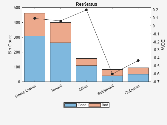
Update the creditscorecard object using the newdata and plot the bins for a later comparison.
scnew = creditscorecard(newdata,'IDVar','CustID');
[bi,cg] = bininfo(scnew,Predictor)
bi=6×6 table
         Bin          Good    Bad     Odds       WOE       InfoValue
    ______________    ____    ___    ______    ________    _________

    {'Home Owner'}    308     154         2    0.092373    0.0032392
    {'Tenant'    }    264     136    1.9412     0.06252    0.0012907
    {'Other'     }    109      49    2.2245     0.19875    0.0050386
    {'Subtenant' }     42      42         1    -0.60077     0.026813
    {'CoOwner'   }     52      44    1.1818    -0.43372     0.015802
    {'Totals'    }    775     425    1.8235         NaN     0.052183
cg=5×2 table
       Category       BinNumber
    ______________    _________

    {'Home Owner'}        1
    {'Tenant'    }        2
    {'Other'     }        3
    {'Subtenant' }        4
    {'CoOwner'   }        5
plotbins(scnew,Predictor)
Perform automatic binning for the categorical Predictor using the default Monotone algorithm with the AlgorithmOptions name-value pair arguments for 'SortCategories' and 'Trend'.
AlgoOptions = {'SortCategories','Goods','Trend','Increasing'};

scnew = autobinning(scnew,Predictor,'Algorithm','Monotone',...
    'AlgorithmOptions',AlgoOptions);
Use bininfo to display the bin information. The second output parameter 'cg' captures the bin membership, which is the bin number that each group belongs to.
[bi,cg] = bininfo(scnew,Predictor)
bi=4×6 table
       Bin        Good    Bad     Odds       WOE       InfoValue
    __________    ____    ___    ______    ________    _________

    {'Group1'}     42      42         1    -0.60077     0.026813
    {'Group2'}     52      44    1.1818    -0.43372     0.015802
    {'Group3'}    681     339    2.0088    0.096788    0.0078459
    {'Totals'}    775     425    1.8235         NaN      0.05046
cg=5×2 table
       Category       BinNumber
    ______________    _________

    {'Subtenant' }        1
    {'CoOwner'   }        2
    {'Other'     }        3
    {'Tenant'    }        3
    {'Home Owner'}        3
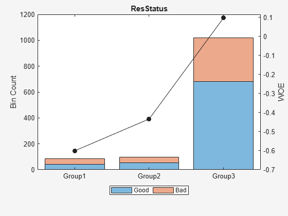
Plot bins and compare with the histogram plotted pre-binning.
plotbins(scnew,Predictor)
Create a creditscorecard object using the CreditCardData.mat file to load the dataMissing with missing values.
load CreditCardData.mat
head(dataMissing,5)
CustID CustAge TmAtAddress ResStatus EmpStatus CustIncome TmWBank OtherCC AMBalance UtilRate status
______ _______ ___________ ___________ _________ __________ _______ _______ _________ ________ ______
1 53 62 <undefined> Unknown 50000 55 Yes 1055.9 0.22 0
2 61 22 Home Owner Employed 52000 25 Yes 1161.6 0.24 0
3 47 30 Tenant Employed 37000 61 No 877.23 0.29 0
4 NaN 75 Home Owner Employed 53000 20 Yes 157.37 0.08 0
5 68 56 Home Owner Employed 53000 14 Yes 561.84 0.11 0
fprintf('Number of rows: %d\n',height(dataMissing))Number of rows: 1200
fprintf('Number of missing values CustAge: %d\n',sum(ismissing(dataMissing.CustAge)))Number of missing values CustAge: 30
fprintf('Number of missing values ResStatus: %d\n',sum(ismissing(dataMissing.ResStatus)))Number of missing values ResStatus: 40
Use creditscorecard with the name-value argument 'BinMissingData' set to true to bin the missing numeric and categorical data in a separate bin.
sc = creditscorecard(dataMissing,'BinMissingData',true);
disp(sc)
creditscorecard with properties:
GoodLabel: 0
ResponseVar: 'status'
WeightsVar: ''
VarNames: {'CustID' 'CustAge' 'TmAtAddress' 'ResStatus' 'EmpStatus' 'CustIncome' 'TmWBank' 'OtherCC' 'AMBalance' 'UtilRate' 'status'}
NumericPredictors: {'CustID' 'CustAge' 'TmAtAddress' 'CustIncome' 'TmWBank' 'AMBalance' 'UtilRate'}
CategoricalPredictors: {'ResStatus' 'EmpStatus' 'OtherCC'}
BinMissingData: 1
IDVar: ''
PredictorVars: {'CustID' 'CustAge' 'TmAtAddress' 'ResStatus' 'EmpStatus' 'CustIncome' 'TmWBank' 'OtherCC' 'AMBalance' 'UtilRate'}
Data: [1200×11 table]
Perform automatic binning using the Merge algorithm.
sc = autobinning(sc,'Algorithm','Merge');
Display bin information for numeric data for 'CustAge' that includes missing data in a separate bin labelled <missing> and this is the last bin. No matter what binning algorithm is used in autobinning, the algorithm operates on the non-missing data and the bin for the <missing> numeric values for a predictor is always the last bin.
[bi,cp] = bininfo(sc,'CustAge');
disp(bi)
Bin Good Bad Odds WOE InfoValue
_____________ ____ ___ _______ ________ __________
{'[-Inf,32)'} 56 39 1.4359 -0.34263 0.0097643
{'[32,33)' } 13 13 1 -0.70442 0.011663
{'[33,34)' } 9 11 0.81818 -0.90509 0.014934
{'[34,65)' } 677 317 2.1356 0.054351 0.002424
{'[65,Inf]' } 29 6 4.8333 0.87112 0.018295
{'<missing>'} 19 11 1.7273 -0.15787 0.00063885
{'Totals' } 803 397 2.0227 NaN 0.057718
plotbins(sc,'CustAge')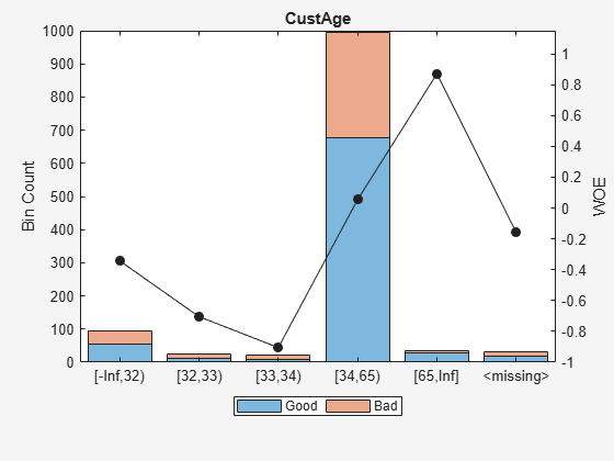
Display bin information for categorical data for 'ResStatus' that includes missing data in a separate bin labelled <missing> and this is the last bin. No matter what binning algorithm is used in autobinning, the algorithm operates on the non-missing data and the bin for the <missing> categorical values for a predictor is always the last bin.
[bi,cg] = bininfo(sc,'ResStatus');
disp(bi)
Bin Good Bad Odds WOE InfoValue
_____________ ____ ___ ______ _________ __________
{'Group1' } 648 332 1.9518 -0.035663 0.0010449
{'Group2' } 128 52 2.4615 0.19637 0.0055808
{'<missing>'} 27 13 2.0769 0.026469 2.3248e-05
{'Totals' } 803 397 2.0227 NaN 0.0066489
plotbins(sc,'ResStatus')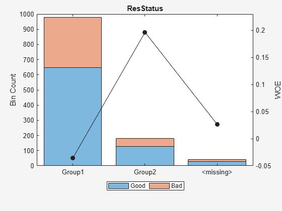
This example demonstrates using the 'Split' algorithm with categorical and numeric predictors. Load the CreditCardData.mat dataset and modify so that it contains four categories for the predictor 'ResStatus' to demonstrate how the split algorithm works.
load CreditCardData.mat
x = data.ResStatus;
Ind = find(x == 'Tenant');
Nx  = length(Ind);
x(Ind(1:floor(Nx/3))) = 'Subletter';
data.ResStatus = x;
Create a creditscorecard and use bininfo to display the 'Statistics'.
sc = creditscorecard(data,'IDVar','CustID');
[bi1,cg1] = bininfo(sc,'ResStatus','Statistics',{'Odds','WOE','InfoValue'});
disp(bi1)
         Bin          Good    Bad     Odds        WOE       InfoValue
    ______________    ____    ___    ______    _________    __________

    {'Home Owner'}    365     177    2.0621     0.019329     0.0001682
    {'Tenant'    }    204     112    1.8214      -0.1048     0.0029415
    {'Other'     }    131      53    2.4717      0.20049     0.0059418
    {'Subletter' }    103      55    1.8727    -0.077023    0.00079103
    {'Totals'    }    803     397    2.0227          NaN     0.0098426
disp(cg1)
       Category       BinNumber
    ______________    _________

    {'Home Owner'}        1
    {'Tenant'    }        2
    {'Other'     }        3
    {'Subletter' }        4
Using the Split Algorithm with a Categorical Predictor
Apply presorting to the 'ResStatus' category using the default sorting by 'Odds' and specify the 'Split' algorithm.
sc = autobinning(sc,'ResStatus', 'Algorithm', 'split','AlgorithmOptions',...
    {'Measure','gini','SortCategories','odds','Tolerance',1e4});
[bi2,cg2] = bininfo(sc,'ResStatus','Statistics',{'Odds','WOE','InfoValue'});
disp(bi2)
       Bin        Good    Bad     Odds     WOE    InfoValue
    __________    ____    ___    ______    ___    _________

    {'Group1'}    803     397    2.0227      0        0
    {'Totals'}    803     397    2.0227    NaN        0
disp(cg2)
       Category       BinNumber
    ______________    _________

    {'Tenant'    }        1
    {'Subletter' }        1
    {'Home Owner'}        1
    {'Other'     }        1
Using the Split Algorithm with a Numeric Predictor
To demonstrate a split for the numeric predictor, 'TmAtAddress', first use autobinning with the default 'Monotone' algorithm.
sc = autobinning(sc,'TmAtAddress');
bi3 = bininfo(sc,'TmAtAddress','Statistics',{'Odds','WOE','InfoValue'});
disp(bi3)
         Bin         Good    Bad     Odds        WOE       InfoValue
    _____________    ____    ___    ______    _________    __________

    {'[-Inf,23)'}    239     129    1.8527    -0.087767     0.0023963
    {'[23,83)'  }    480     232     2.069      0.02263    0.00030269
    {'[83,Inf]' }     84      36    2.3333      0.14288       0.00199
    {'Totals'   }    803     397    2.0227          NaN      0.004689
Then use autobinning with the 'Split' algorithm.
sc = autobinning(sc,'TmAtAddress','Algorithm', 'Split');
bi4 = bininfo(sc,'TmAtAddress','Statistics',{'Odds','WOE','InfoValue'});
disp(bi4)
        Bin         Good    Bad     Odds         WOE       InfoValue
    ____________    ____    ___    _______    _________    __________

    {'[-Inf,4)'}     20      12     1.6667     -0.19359     0.0010299
    {'[4,5)'   }      4       7    0.57143       -1.264      0.015991
    {'[5,23)'  }    215     110     1.9545    -0.034261    0.00031973
    {'[23,33)' }    130      39     3.3333      0.49955        0.0318
    {'[33,Inf]'}    434     229     1.8952    -0.065096     0.0023664
    {'Totals'  }    803     397     2.0227          NaN      0.051507
Load the CreditCardData.mat dataset. This example demonstrates using the 'Merge' algorithm with categorical and numeric predictors.
load CreditCardData.matUsing the Merge Algorithm with a Categorical Predictor
To merge a categorical predictor, create a creditscorecard using default sorting by 'Odds' and then use bininfo on the categorical predictor 'ResStatus'.
sc = creditscorecard(data,'IDVar','CustID');
[bi1,cg1] = bininfo(sc,'ResStatus','Statistics',{'Odds','WOE','InfoValue'});
disp(bi1);
         Bin          Good    Bad     Odds        WOE       InfoValue
    ______________    ____    ___    ______    _________    _________

    {'Home Owner'}    365     177    2.0621     0.019329    0.0001682
    {'Tenant'    }    307     167    1.8383    -0.095564    0.0036638
    {'Other'     }    131      53    2.4717      0.20049    0.0059418
    {'Totals'    }    803     397    2.0227          NaN    0.0097738
disp(cg1);
       Category       BinNumber
    ______________    _________

    {'Home Owner'}        1
    {'Tenant'    }        2
    {'Other'     }        3
Use autobinning and specify the 'Merge' algorithm.
sc = autobinning(sc,'ResStatus','Algorithm', 'Merge');
[bi2,cg2] = bininfo(sc,'ResStatus','Statistics',{'Odds','WOE','InfoValue'});
disp(bi2)
       Bin        Good    Bad     Odds        WOE       InfoValue
    __________    ____    ___    ______    _________    _________

    {'Group1'}    672     344    1.9535    -0.034802    0.0010314
    {'Group2'}    131      53    2.4717      0.20049    0.0059418
    {'Totals'}    803     397    2.0227          NaN    0.0069732
disp(cg2)
       Category       BinNumber
    ______________    _________

    {'Tenant'    }        1
    {'Home Owner'}        1
    {'Other'     }        2
Using the Merge Algorithm with a Numeric Predictor
To demonstrate a merge for the numeric predictor, 'TmAtAddress', first use autobinning with the default 'Monotone' algorithm.
sc = autobinning(sc,'TmAtAddress');
bi3 = bininfo(sc,'TmAtAddress','Statistics',{'Odds','WOE','InfoValue'});
disp(bi3)
         Bin         Good    Bad     Odds        WOE       InfoValue
    _____________    ____    ___    ______    _________    __________

    {'[-Inf,23)'}    239     129    1.8527    -0.087767     0.0023963
    {'[23,83)'  }    480     232     2.069      0.02263    0.00030269
    {'[83,Inf]' }     84      36    2.3333      0.14288       0.00199
    {'Totals'   }    803     397    2.0227          NaN      0.004689
Then use autobinning with the 'Merge' algorithm.
sc = autobinning(sc,'TmAtAddress','Algorithm', 'Merge');
bi4 = bininfo(sc,'TmAtAddress','Statistics',{'Odds','WOE','InfoValue'});
disp(bi4)
         Bin         Good    Bad     Odds         WOE       InfoValue
    _____________    ____    ___    _______    _________    __________

    {'[-Inf,28)'}    303     152     1.9934    -0.014566    8.0646e-05
    {'[28,30)'  }     27       2       13.5       1.8983      0.054264
    {'[30,98)'  }    428     216     1.9815    -0.020574    0.00022794
    {'[98,106)' }     11      13    0.84615     -0.87147      0.016599
    {'[106,Inf]'}     34      14     2.4286      0.18288     0.0012942
    {'Totals'   }    803     397     2.0227          NaN      0.072466
Input Arguments
Name-Value Arguments
Output Arguments
More About
References
[1] Anderson, R. The Credit Scoring Toolkit. Oxford University Press, 2007.
[2] Kerber, R. "ChiMerge: Discretization of Numeric Attributes." AAAI-92 Proceedings. 1992.
[3] Liu, H., et. al. Data Mining, Knowledge, and Discovery. Vol 6. Issue 4. October 2002, pp. 393-423.
[4] Refaat, M. Data Preparation for Data Mining Using SAS. Morgan Kaufmann, 2006.
[5] Refaat, M. Credit Risk Scorecards: Development and Implementation Using SAS. lulu.com, 2011.
[6] Thomas, L., et al. Credit Scoring and Its Applications. Society for Industrial and Applied Mathematics, 2002.
Version History
Introduced in R2014b
See Also
creditscorecard | bininfo | predictorinfo | modifypredictor | modifybins | bindata | plotbins | fitmodel | displaypoints | formatpoints | score | setmodel | probdefault | validatemodel