score
Compute credit scores for given data
Syntax
Description
Scores = score(sc)creditscorecard object’s
training data. This data can be a “training” or a
“live” dataset. If the data input argument is
not explicitly provided, the score function determines scores
for the existing creditscorecard object’s data.
formatpoints supports multiple
alternatives to modify the scaling of the scores and can also be used to control
the rounding of points and scores, and whether the base points are reported
separately or spread across predictors. Missing data translates into
NaN values for the corresponding points, and therefore
for the total score. Use formatpoints to modify the
score behavior for rows with missing data.
Scores = score(sc, data)data. This
data can be a “training” or a “live” dataset.
formatpoints supports multiple
alternatives to modify the scaling of the scores and can also be used to control
the rounding of points and scores, and whether the base points are reported
separately or spread across predictors. Missing data translates into
NaN values for the corresponding points, and therefore
for the total score. Use formatpoints to modify the
score behavior for rows with missing data.
[ computes the credit scores and points
for the given data. If the Scores,Points]
= score(sc)data input argument is not
explicitly provided, the score function determines scores for
the existing creditscorecard object’s data.
formatpoints supports multiple
alternatives to modify the scaling of the scores and can also be used to control
the rounding of points and scores, and whether the base points are reported
separately or spread across predictors. Missing data translates into
NaN values for the corresponding points, and therefore
for the total score. Use formatpoints to modify the
score behavior for rows with missing data.
[ computes the
credit scores and points for the given input Scores,Points]
= score(sc,data)data. This
data can be a “training” or a “live” dataset.
formatpoints supports multiple
alternatives to modify the scaling of the scores and can also be used to control
the rounding of points and scores, and whether the base points are reported
separately or spread across predictors. Missing data translates into
NaN values for the corresponding points, and therefore
for the total score. Use formatpoints to modify the
score behavior for rows with missing data.
Examples
This example shows how to use score to obtain scores for the training data.
Create a creditscorecard object using the CreditCardData.mat file to load the data (using a dataset from Refaat 2011). Use the 'IDVar' argument in creditscorecard to indicate that 'CustID' contains ID information and should not be included as a predictor variable.
load CreditCardData sc = creditscorecard(data,'IDVar','CustID');
Perform automatic binning to bin for all predictors.
sc = autobinning(sc);
Fit a linear regression model using default parameters.
sc = fitmodel(sc);
1. Adding CustIncome, Deviance = 1490.8527, Chi2Stat = 32.588614, PValue = 1.1387992e-08
2. Adding TmWBank, Deviance = 1467.1415, Chi2Stat = 23.711203, PValue = 1.1192909e-06
3. Adding AMBalance, Deviance = 1455.5715, Chi2Stat = 11.569967, PValue = 0.00067025601
4. Adding EmpStatus, Deviance = 1447.3451, Chi2Stat = 8.2264038, PValue = 0.0041285257
5. Adding CustAge, Deviance = 1441.994, Chi2Stat = 5.3511754, PValue = 0.020708306
6. Adding ResStatus, Deviance = 1437.8756, Chi2Stat = 4.118404, PValue = 0.042419078
7. Adding OtherCC, Deviance = 1433.707, Chi2Stat = 4.1686018, PValue = 0.041179769
Generalized linear regression model:
logit(status) ~ 1 + CustAge + ResStatus + EmpStatus + CustIncome + TmWBank + OtherCC + AMBalance
Distribution = Binomial
Estimated Coefficients:
Estimate SE tStat pValue
________ ________ ______ __________
(Intercept) 0.70239 0.064001 10.975 5.0538e-28
CustAge 0.60833 0.24932 2.44 0.014687
ResStatus 1.377 0.65272 2.1097 0.034888
EmpStatus 0.88565 0.293 3.0227 0.0025055
CustIncome 0.70164 0.21844 3.2121 0.0013179
TmWBank 1.1074 0.23271 4.7589 1.9464e-06
OtherCC 1.0883 0.52912 2.0569 0.039696
AMBalance 1.045 0.32214 3.2439 0.0011792
1200 observations, 1192 error degrees of freedom
Dispersion: 1
Chi^2-statistic vs. constant model: 89.7, p-value = 1.4e-16
Score training data using the score function without an optional input for data. By default, it returns unscaled scores. For brevity, only the first ten scores are displayed.
Scores = score(sc); disp(Scores(1:10))
1.0968
1.4646
0.7662
1.5779
1.4535
1.8944
-0.0872
0.9207
1.0399
0.8252
Scale scores and display both points and scores for each individual in the training data (for brevity, only the first ten rows are displayed). For other scaling methods, and other options for formatting points and scores, use the formatpoints function.
sc = formatpoints(sc,'WorstAndBestScores',[300 850]);
[Scores,Points] = score(sc);
disp(Scores(1:10))602.0394 648.1988 560.5569 662.4189 646.8109 702.1398 453.4572 579.9475 594.9064 567.9533
disp(Points(1:10,:))
CustAge ResStatus EmpStatus CustIncome TmWBank OtherCC AMBalance
_______ _________ _________ __________ _______ _______ _________
95.256 62.421 56.765 121.18 116.05 86.224 64.15
126.46 82.276 105.81 121.18 62.107 86.224 64.15
93.256 62.421 105.81 76.585 116.05 42.287 64.15
95.256 82.276 105.81 121.18 60.719 86.224 110.96
126.46 82.276 105.81 121.18 60.719 86.224 64.15
126.46 82.276 105.81 121.18 116.05 86.224 64.15
48.727 82.276 56.765 53.208 62.107 86.224 64.15
95.256 113.58 105.81 121.18 62.107 42.287 39.729
95.256 62.421 56.765 121.18 62.107 86.224 110.96
95.256 82.276 56.765 121.18 62.107 86.224 64.15
This example describes the assignment of points for missing data when the 'BinMissingData' option is set to true.
Predictors that have missing data in the training set have an explicit bin for
<missing>with corresponding points in the final scorecard. These points are computed from the Weight-of-Evidence (WOE) value for the<missing>bin and the logistic model coefficients. For scoring purposes, these points are assigned to missing values and to out-of-range values.Predictors with no missing data in the training set have no
<missing>bin, therefore no WOE can be estimated from the training data. By default, the points for missing and out-of-range values are set toNaN, and this leads to a score ofNaNwhen runningscore. For predictors that have no explicit<missing>bin, use the name-value argument'Missing'informatpointsto indicate how missing data should be treated for scoring purposes.
Create a creditscorecard object using the CreditCardData.mat file to load the dataMissing with missing values.
load CreditCardData.mat
head(dataMissing,5) CustID CustAge TmAtAddress ResStatus EmpStatus CustIncome TmWBank OtherCC AMBalance UtilRate status
______ _______ ___________ ___________ _________ __________ _______ _______ _________ ________ ______
1 53 62 <undefined> Unknown 50000 55 Yes 1055.9 0.22 0
2 61 22 Home Owner Employed 52000 25 Yes 1161.6 0.24 0
3 47 30 Tenant Employed 37000 61 No 877.23 0.29 0
4 NaN 75 Home Owner Employed 53000 20 Yes 157.37 0.08 0
5 68 56 Home Owner Employed 53000 14 Yes 561.84 0.11 0
fprintf('Number of rows: %d\n',height(dataMissing))Number of rows: 1200
fprintf('Number of missing values CustAge: %d\n',sum(ismissing(dataMissing.CustAge)))Number of missing values CustAge: 30
fprintf('Number of missing values ResStatus: %d\n',sum(ismissing(dataMissing.ResStatus)))Number of missing values ResStatus: 40
Use creditscorecard with the name-value argument 'BinMissingData' set to true to bin the missing numeric or categorical data in a separate bin. Apply automatic binning.
sc = creditscorecard(dataMissing,'IDVar','CustID','BinMissingData',true); sc = autobinning(sc); disp(sc)
creditscorecard with properties:
GoodLabel: 0
ResponseVar: 'status'
WeightsVar: ''
VarNames: {'CustID' 'CustAge' 'TmAtAddress' 'ResStatus' 'EmpStatus' 'CustIncome' 'TmWBank' 'OtherCC' 'AMBalance' 'UtilRate' 'status'}
NumericPredictors: {'CustAge' 'TmAtAddress' 'CustIncome' 'TmWBank' 'AMBalance' 'UtilRate'}
CategoricalPredictors: {'ResStatus' 'EmpStatus' 'OtherCC'}
BinMissingData: 1
IDVar: 'CustID'
PredictorVars: {'CustAge' 'TmAtAddress' 'ResStatus' 'EmpStatus' 'CustIncome' 'TmWBank' 'OtherCC' 'AMBalance' 'UtilRate'}
Data: [1200×11 table]
Set a minimum value of zero for CustAge and CustIncome. With this, any negative age or income information becomes invalid or "out-of-range". For scoring purposes, out-of-range values are given the same points as missing values.
sc = modifybins(sc,'CustAge','MinValue',0); sc = modifybins(sc,'CustIncome','MinValue',0);
Display and plot bin information for numeric data for 'CustAge' that includes missing data in a separate bin labelled <missing>.
[bi,cp] = bininfo(sc,'CustAge');
disp(bi) Bin Good Bad Odds WOE InfoValue
_____________ ____ ___ ______ ________ __________
{'[0,33)' } 69 52 1.3269 -0.42156 0.018993
{'[33,37)' } 63 45 1.4 -0.36795 0.012839
{'[37,40)' } 72 47 1.5319 -0.2779 0.0079824
{'[40,46)' } 172 89 1.9326 -0.04556 0.0004549
{'[46,48)' } 59 25 2.36 0.15424 0.0016199
{'[48,51)' } 99 41 2.4146 0.17713 0.0035449
{'[51,58)' } 157 62 2.5323 0.22469 0.0088407
{'[58,Inf]' } 93 25 3.72 0.60931 0.032198
{'<missing>'} 19 11 1.7273 -0.15787 0.00063885
{'Totals' } 803 397 2.0227 NaN 0.087112
plotbins(sc,'CustAge')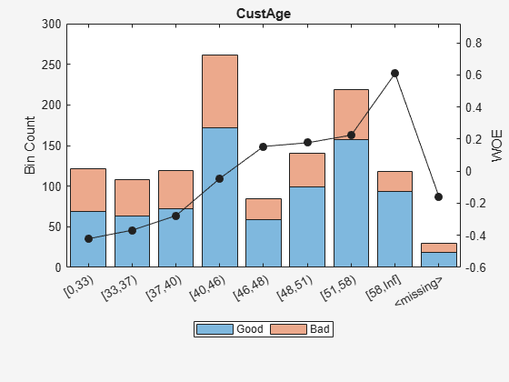
Display and plot bin information for categorical data for 'ResStatus' that includes missing data in a separate bin labelled <missing>.
[bi,cg] = bininfo(sc,'ResStatus');
disp(bi) Bin Good Bad Odds WOE InfoValue
______________ ____ ___ ______ _________ __________
{'Tenant' } 296 161 1.8385 -0.095463 0.0035249
{'Home Owner'} 352 171 2.0585 0.017549 0.00013382
{'Other' } 128 52 2.4615 0.19637 0.0055808
{'<missing>' } 27 13 2.0769 0.026469 2.3248e-05
{'Totals' } 803 397 2.0227 NaN 0.0092627
plotbins(sc,'ResStatus')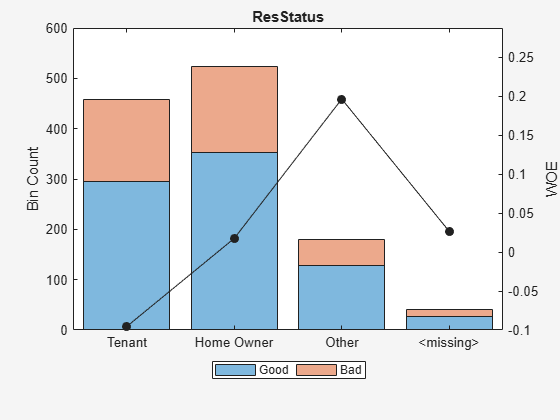
For the 'CustAge' and 'ResStatus' predictors, there is missing data (NaNs and <undefined>) in the training data, and the binning process estimates a WOE value of -0.15787 and 0.026469 respectively for missing data in these predictors, as shown above.
For EmpStatus and CustIncome there is no explicit bin for missing values because the training data has no missing values for these predictors.
bi = bininfo(sc,'EmpStatus');
disp(bi) Bin Good Bad Odds WOE InfoValue
____________ ____ ___ ______ ________ _________
{'Unknown' } 396 239 1.6569 -0.19947 0.021715
{'Employed'} 407 158 2.5759 0.2418 0.026323
{'Totals' } 803 397 2.0227 NaN 0.048038
bi = bininfo(sc,'CustIncome');
disp(bi) Bin Good Bad Odds WOE InfoValue
_________________ ____ ___ _______ _________ __________
{'[0,29000)' } 53 58 0.91379 -0.79457 0.06364
{'[29000,33000)'} 74 49 1.5102 -0.29217 0.0091366
{'[33000,35000)'} 68 36 1.8889 -0.06843 0.00041042
{'[35000,40000)'} 193 98 1.9694 -0.026696 0.00017359
{'[40000,42000)'} 68 34 2 -0.011271 1.0819e-05
{'[42000,47000)'} 164 66 2.4848 0.20579 0.0078175
{'[47000,Inf]' } 183 56 3.2679 0.47972 0.041657
{'Totals' } 803 397 2.0227 NaN 0.12285
Use fitmodel to fit a logistic regression model using Weight of Evidence (WOE) data. fitmodel internally transforms all the predictor variables into WOE values, using the bins found with the automatic binning process. fitmodel then fits a logistic regression model using a stepwise method (by default). For predictors that have missing data, there is an explicit <missing> bin, with a corresponding WOE value computed from the data. When using fitmodel, the corresponding WOE value for the <missing> bin is applied when performing the WOE transformation.
[sc,mdl] = fitmodel(sc);
1. Adding CustIncome, Deviance = 1490.8527, Chi2Stat = 32.588614, PValue = 1.1387992e-08
2. Adding TmWBank, Deviance = 1467.1415, Chi2Stat = 23.711203, PValue = 1.1192909e-06
3. Adding AMBalance, Deviance = 1455.5715, Chi2Stat = 11.569967, PValue = 0.00067025601
4. Adding EmpStatus, Deviance = 1447.3451, Chi2Stat = 8.2264038, PValue = 0.0041285257
5. Adding CustAge, Deviance = 1442.8477, Chi2Stat = 4.4974731, PValue = 0.033944979
6. Adding ResStatus, Deviance = 1438.9783, Chi2Stat = 3.86941, PValue = 0.049173805
7. Adding OtherCC, Deviance = 1434.9751, Chi2Stat = 4.0031966, PValue = 0.045414057
Generalized linear regression model:
logit(status) ~ 1 + CustAge + ResStatus + EmpStatus + CustIncome + TmWBank + OtherCC + AMBalance
Distribution = Binomial
Estimated Coefficients:
Estimate SE tStat pValue
________ ________ ______ __________
(Intercept) 0.70229 0.063959 10.98 4.7498e-28
CustAge 0.57421 0.25708 2.2335 0.025513
ResStatus 1.3629 0.66952 2.0356 0.04179
EmpStatus 0.88373 0.2929 3.0172 0.002551
CustIncome 0.73535 0.2159 3.406 0.00065929
TmWBank 1.1065 0.23267 4.7556 1.9783e-06
OtherCC 1.0648 0.52826 2.0156 0.043841
AMBalance 1.0446 0.32197 3.2443 0.0011775
1200 observations, 1192 error degrees of freedom
Dispersion: 1
Chi^2-statistic vs. constant model: 88.5, p-value = 2.55e-16
Scale the scorecard points by the "points, odds, and points to double the odds (PDO)" method using the 'PointsOddsAndPDO' argument of formatpoints. Suppose that you want a score of 500 points to have odds of 2 (twice as likely to be good than to be bad) and that the odds double every 50 points (so that 550 points would have odds of 4).
Display the scorecard showing the scaled points for predictors retained in the fitting model.
sc = formatpoints(sc,'PointsOddsAndPDO',[500 2 50]);
PointsInfo = displaypoints(sc)PointsInfo=38×3 table
Predictors Bin Points
_____________ ______________ ______
{'CustAge' } {'[0,33)' } 54.062
{'CustAge' } {'[33,37)' } 56.282
{'CustAge' } {'[37,40)' } 60.012
{'CustAge' } {'[40,46)' } 69.636
{'CustAge' } {'[46,48)' } 77.912
{'CustAge' } {'[48,51)' } 78.86
{'CustAge' } {'[51,58)' } 80.83
{'CustAge' } {'[58,Inf]' } 96.76
{'CustAge' } {'<missing>' } 64.984
{'ResStatus'} {'Tenant' } 62.138
{'ResStatus'} {'Home Owner'} 73.248
{'ResStatus'} {'Other' } 90.828
{'ResStatus'} {'<missing>' } 74.125
{'EmpStatus'} {'Unknown' } 58.807
{'EmpStatus'} {'Employed' } 86.937
{'EmpStatus'} {'<missing>' } NaN
⋮
Notice that points for the <missing> bin for CustAge and ResStatus are explicitly shown (as 64.9836 and 74.1250, respectively). These points are computed from the WOE value for the <missing> bin, and the logistic model coefficients.
For predictors that have no missing data in the training set, there is no explicit <missing> bin. By default the points are set to NaN for missing data and they lead to a score of NaN when running score. For predictors that have no explicit <missing> bin, use the name-value argument 'Missing' in formatpoints to indicate how missing data should be treated for scoring purposes.
For the purpose of illustration, take a few rows from the original data as test data and introduce some missing data. Also introduce some invalid, or out-of-range values. For numeric data, values below the minimum (or above the maximum) allowed are considered invalid, such as a negative value for age (recall 'MinValue' was earlier set to 0 for CustAge and CustIncome). For categorical data, invalid values are categories not explicitly included in the scorecard, for example, a residential status not previously mapped to scorecard categories, such as "House", or a meaningless string such as "abc123".
tdata = dataMissing(11:18,mdl.PredictorNames); % Keep only the predictors retained in the model % Set some missing values tdata.CustAge(1) = NaN; tdata.ResStatus(2) = missing; tdata.EmpStatus(3) = missing; tdata.CustIncome(4) = NaN; % Set some invalid values tdata.CustAge(5) = -100; tdata.ResStatus(6) = 'House'; tdata.EmpStatus(7) = 'Freelancer'; tdata.CustIncome(8) = -1; disp(tdata)
CustAge ResStatus EmpStatus CustIncome TmWBank OtherCC AMBalance
_______ ___________ ___________ __________ _______ _______ _________
NaN Tenant Unknown 34000 44 Yes 119.8
48 <undefined> Unknown 44000 14 Yes 403.62
65 Home Owner <undefined> 48000 6 No 111.88
44 Other Unknown NaN 35 No 436.41
-100 Other Employed 46000 16 Yes 162.21
33 House Employed 36000 36 Yes 845.02
39 Tenant Freelancer 34000 40 Yes 756.26
24 Home Owner Employed -1 19 Yes 449.61
Score the new data and see how points are assigned for missing CustAge and ResStatus, because we have an explicit bin with points for <missing>. However, for EmpStatus and CustIncome the score function sets the points to NaN.
[Scores,Points] = score(sc,tdata); disp(Scores)
481.2231
520.8353
NaN
NaN
551.7922
487.9588
NaN
NaN
disp(Points)
CustAge ResStatus EmpStatus CustIncome TmWBank OtherCC AMBalance
_______ _________ _________ __________ _______ _______ _________
64.984 62.138 58.807 67.893 61.858 75.622 89.922
78.86 74.125 58.807 82.439 61.061 75.622 89.922
96.76 73.248 NaN 96.969 51.132 50.914 89.922
69.636 90.828 58.807 NaN 61.858 50.914 89.922
64.984 90.828 86.937 82.439 61.061 75.622 89.922
56.282 74.125 86.937 70.107 61.858 75.622 63.028
60.012 62.138 NaN 67.893 61.858 75.622 63.028
54.062 73.248 86.937 NaN 61.061 75.622 89.922
Use the name-value argument 'Missing' in formatpoints to choose how to assign points to missing values for predictors that do not have an explicit <missing> bin. In this example, use the 'MinPoints' option for the 'Missing' argument. The minimum points for EmpStatus in the scorecard displayed above are 58.8072, and for CustIncome the minimum points are 29.3753.
sc = formatpoints(sc,'Missing','MinPoints'); [Scores,Points] = score(sc,tdata); disp(Scores)
481.2231 520.8353 517.7532 451.3405 551.7922 487.9588 449.3577 470.2267
disp(Points)
CustAge ResStatus EmpStatus CustIncome TmWBank OtherCC AMBalance
_______ _________ _________ __________ _______ _______ _________
64.984 62.138 58.807 67.893 61.858 75.622 89.922
78.86 74.125 58.807 82.439 61.061 75.622 89.922
96.76 73.248 58.807 96.969 51.132 50.914 89.922
69.636 90.828 58.807 29.375 61.858 50.914 89.922
64.984 90.828 86.937 82.439 61.061 75.622 89.922
56.282 74.125 86.937 70.107 61.858 75.622 63.028
60.012 62.138 58.807 67.893 61.858 75.622 63.028
54.062 73.248 86.937 29.375 61.061 75.622 89.922
This example shows how to use score to obtain scores for a new dataset (for example, a validation or a test dataset) using the optional 'data' input in the score function.
Create a creditscorecard object using the CreditCardData.mat file to load the data (using a dataset from Refaat 2011). Use the 'IDVar' argument in creditscorecard to indicate that 'CustID' contains ID information and should not be included as a predictor variable.
load CreditCardData
sc = creditscorecard(data,'IDVar','CustID');
Perform automatic binning to bin for all predictors.
sc = autobinning(sc);
Fit a linear regression model using default parameters.
sc = fitmodel(sc);
1. Adding CustIncome, Deviance = 1490.8527, Chi2Stat = 32.588614, PValue = 1.1387992e-08
2. Adding TmWBank, Deviance = 1467.1415, Chi2Stat = 23.711203, PValue = 1.1192909e-06
3. Adding AMBalance, Deviance = 1455.5715, Chi2Stat = 11.569967, PValue = 0.00067025601
4. Adding EmpStatus, Deviance = 1447.3451, Chi2Stat = 8.2264038, PValue = 0.0041285257
5. Adding CustAge, Deviance = 1441.994, Chi2Stat = 5.3511754, PValue = 0.020708306
6. Adding ResStatus, Deviance = 1437.8756, Chi2Stat = 4.118404, PValue = 0.042419078
7. Adding OtherCC, Deviance = 1433.707, Chi2Stat = 4.1686018, PValue = 0.041179769

Generalized linear regression model:
    logit(status) ~ 1 + CustAge + ResStatus + EmpStatus + CustIncome + TmWBank + OtherCC + AMBalance
    Distribution = Binomial

Estimated Coefficients:
                   Estimate       SE       tStat       pValue
                   ________    ________    ______    __________

    (Intercept)    0.70239     0.064001    10.975    5.0538e-28
    CustAge        0.60833      0.24932      2.44      0.014687
    ResStatus        1.377      0.65272    2.1097      0.034888
    EmpStatus      0.88565        0.293    3.0227     0.0025055
    CustIncome     0.70164      0.21844    3.2121     0.0013179
    TmWBank         1.1074      0.23271    4.7589    1.9464e-06
    OtherCC         1.0883      0.52912    2.0569      0.039696
    AMBalance        1.045      0.32214    3.2439     0.0011792


1200 observations, 1192 error degrees of freedom
Dispersion: 1
Chi^2-statistic vs. constant model: 89.7, p-value = 1.4e-16
For the purpose of illustration, suppose that a few rows from the original data are our "new" data. Use the optional data input argument in the score function to obtain the scores for the newdata.
newdata = data(10:20,:);
Scores = score(sc,newdata)
Scores = 11×1

    0.8252
    0.6553
    1.2443
    0.9478
    0.5690
    1.6192
    0.4899
    0.3824
    0.2945
    1.4401
    0.8242
Input Arguments
Output Arguments
Algorithms
The score of an individual i is given by the formula
Score(i) = Shift + Slope*(b0 + b1*WOE1(i) + b2*WOE2(i)+ ... +bp*WOEp(i))
where bj is the coefficient of the j-th variable
in the model, and WOEj(i) is the Weight of
Evidence (WOE) value for the i-th individual corresponding to the
j-th model variable. Shift and
Slope are scaling constants that can be controlled with formatpoints.
If the data for individual i is in the i-th row
of a given dataset, to compute a score, the
data(i,j) is binned using existing binning
maps, and converted into a corresponding Weight of Evidence value
WOEj(i). Using the model
coefficients, the unscaled score is computed
as
s = b0 + b1*WOE1(i) + ... +bp*WOEp(i).
For simplicity, assume in the description above that the j-th variable in the model is the j-th column in the data input, although, in general, the order of variables in a given dataset does not have to match the order of variables in the model, and the dataset could have additional variables that are not used in the model.
The formatting options can be controlled using formatpoints.
References
[1] Anderson, R. The Credit Scoring Toolkit. Oxford University Press, 2007.
[2] Refaat, M. Credit Risk Scorecards: Development and Implementation Using SAS. lulu.com, 2011.
Version History
Introduced in R2014b
See Also
creditscorecard | autobinning | bininfo | predictorinfo | modifypredictor | plotbins | modifybins | bindata | fitmodel | formatpoints | displaypoints | setmodel | probdefault | validatemodel | table