displaypoints
Return points per predictor per bin
Syntax
Description
PointsInfo = displaypoints(sc)creditscorecard object after a linear logistic regression
model is fit using fitmodel to the Weight of
Evidence data. The PointsInfo table displays information on
the predictor name, bin labels, and the corresponding points per bin.
[ returns a table of points for
all bins of all predictor variables used in the
PointsInfo,MinScore,MaxScore]
= displaypoints(sc)creditscorecard object after a linear logistic regression
model is fit (fitmodel) to the Weight of
Evidence data. The PointsInfo table displays information on
the predictor name, bin labels, and the corresponding points per bin and
displaypoints. In addition, the optional
MinScore and MaxScore values are
returned.
[
specifies options using one or more name-value pair arguments in addition to the
input arguments in the previous syntax. PointsInfo,MinScore,MaxScore]
= displaypoints(___,Name,Value)
Examples
This example shows how to use displaypoints after a model is fitted to compute the unscaled points per bin, for a given predictor in the creditscorecard model.
Create a creditscorecard object using the CreditCardData.mat file to load the data (using a dataset from Refaat 2011). Use the 'IDVar' argument in the creditscorecard function to indicate that 'CustID' contains ID information and should not be included as a predictor variable.
load CreditCardData sc = creditscorecard(data,'IDVar','CustID');
Perform automatic binning to bin for all predictors.
sc = autobinning(sc);
Fit a linear regression model using default parameters.
sc = fitmodel(sc);
1. Adding CustIncome, Deviance = 1490.8527, Chi2Stat = 32.588614, PValue = 1.1387992e-08
2. Adding TmWBank, Deviance = 1467.1415, Chi2Stat = 23.711203, PValue = 1.1192909e-06
3. Adding AMBalance, Deviance = 1455.5715, Chi2Stat = 11.569967, PValue = 0.00067025601
4. Adding EmpStatus, Deviance = 1447.3451, Chi2Stat = 8.2264038, PValue = 0.0041285257
5. Adding CustAge, Deviance = 1441.994, Chi2Stat = 5.3511754, PValue = 0.020708306
6. Adding ResStatus, Deviance = 1437.8756, Chi2Stat = 4.118404, PValue = 0.042419078
7. Adding OtherCC, Deviance = 1433.707, Chi2Stat = 4.1686018, PValue = 0.041179769
Generalized linear regression model:
logit(status) ~ 1 + CustAge + ResStatus + EmpStatus + CustIncome + TmWBank + OtherCC + AMBalance
Distribution = Binomial
Estimated Coefficients:
Estimate SE tStat pValue
________ ________ ______ __________
(Intercept) 0.70239 0.064001 10.975 5.0538e-28
CustAge 0.60833 0.24932 2.44 0.014687
ResStatus 1.377 0.65272 2.1097 0.034888
EmpStatus 0.88565 0.293 3.0227 0.0025055
CustIncome 0.70164 0.21844 3.2121 0.0013179
TmWBank 1.1074 0.23271 4.7589 1.9464e-06
OtherCC 1.0883 0.52912 2.0569 0.039696
AMBalance 1.045 0.32214 3.2439 0.0011792
1200 observations, 1192 error degrees of freedom
Dispersion: 1
Chi^2-statistic vs. constant model: 89.7, p-value = 1.4e-16
Display unscaled points for predictors retained in the fitting model.
PointsInfo = displaypoints(sc)
PointsInfo=37×3 table
Predictors Bin Points
______________ ________________ _________
{'CustAge' } {'[-Inf,33)' } -0.15894
{'CustAge' } {'[33,37)' } -0.14036
{'CustAge' } {'[37,40)' } -0.060323
{'CustAge' } {'[40,46)' } 0.046408
{'CustAge' } {'[46,48)' } 0.21445
{'CustAge' } {'[48,58)' } 0.23039
{'CustAge' } {'[58,Inf]' } 0.479
{'CustAge' } {'<missing>' } NaN
{'ResStatus' } {'Tenant' } -0.031252
{'ResStatus' } {'Home Owner' } 0.12696
{'ResStatus' } {'Other' } 0.37641
{'ResStatus' } {'<missing>' } NaN
{'EmpStatus' } {'Unknown' } -0.076317
{'EmpStatus' } {'Employed' } 0.31449
{'EmpStatus' } {'<missing>' } NaN
{'CustIncome'} {'[-Inf,29000)'} -0.45716
⋮
displaypoints always displays a '<missing>' bin for each predictor. The value of the '<missing>' bin comes from the initial creditscorecard object, and the '<missing>' bin is set to NaN whenever the scorecard model has no information on how to assign points to missing data.
To configure the points for the '<missing>' bin, you must use the initial creditscorecard object. For predictors that have missing values in the training set, the points for the '<missing>' bin are estimated from the data if the 'BinMissingData' name-value pair argument is set to true using creditscorecard. When the 'BinMissingData' parameter is set to false, or when the data contains no missing values in the training set, use the 'Missing' name-value pair argument in formatpoints to indicate how to assign points to the missing data.
Create a creditscorecard object using the CreditCardData.mat file to load the data with missing values.
load CreditCardData.mat
head(dataMissing,5) CustID CustAge TmAtAddress ResStatus EmpStatus CustIncome TmWBank OtherCC AMBalance UtilRate status
______ _______ ___________ ___________ _________ __________ _______ _______ _________ ________ ______
1 53 62 <undefined> Unknown 50000 55 Yes 1055.9 0.22 0
2 61 22 Home Owner Employed 52000 25 Yes 1161.6 0.24 0
3 47 30 Tenant Employed 37000 61 No 877.23 0.29 0
4 NaN 75 Home Owner Employed 53000 20 Yes 157.37 0.08 0
5 68 56 Home Owner Employed 53000 14 Yes 561.84 0.11 0
fprintf('Number of rows: %d\n',height(dataMissing))Number of rows: 1200
fprintf('Number of missing values CustAge: %d\n',sum(ismissing(dataMissing.CustAge)))Number of missing values CustAge: 30
fprintf('Number of missing values ResStatus: %d\n',sum(ismissing(dataMissing.ResStatus)))Number of missing values ResStatus: 40
Use creditscorecard with the name-value argument 'BinMissingData' set to true to bin the missing numeric or categorical data in a separate bin. Apply automatic binning.
sc = creditscorecard(dataMissing,'IDVar','CustID','BinMissingData',true); sc = autobinning(sc); disp(sc)
creditscorecard with properties:
GoodLabel: 0
ResponseVar: 'status'
WeightsVar: ''
VarNames: {'CustID' 'CustAge' 'TmAtAddress' 'ResStatus' 'EmpStatus' 'CustIncome' 'TmWBank' 'OtherCC' 'AMBalance' 'UtilRate' 'status'}
NumericPredictors: {'CustAge' 'TmAtAddress' 'CustIncome' 'TmWBank' 'AMBalance' 'UtilRate'}
CategoricalPredictors: {'ResStatus' 'EmpStatus' 'OtherCC'}
BinMissingData: 1
IDVar: 'CustID'
PredictorVars: {'CustAge' 'TmAtAddress' 'ResStatus' 'EmpStatus' 'CustIncome' 'TmWBank' 'OtherCC' 'AMBalance' 'UtilRate'}
Data: [1200×11 table]
Display and plot bin information for numeric data for 'CustAge' that includes missing data in a separate bin labelled <missing>.
[bi,cp] = bininfo(sc,'CustAge');
disp(bi) Bin Good Bad Odds WOE InfoValue
_____________ ____ ___ ______ ________ __________
{'[-Inf,33)'} 69 52 1.3269 -0.42156 0.018993
{'[33,37)' } 63 45 1.4 -0.36795 0.012839
{'[37,40)' } 72 47 1.5319 -0.2779 0.0079824
{'[40,46)' } 172 89 1.9326 -0.04556 0.0004549
{'[46,48)' } 59 25 2.36 0.15424 0.0016199
{'[48,51)' } 99 41 2.4146 0.17713 0.0035449
{'[51,58)' } 157 62 2.5323 0.22469 0.0088407
{'[58,Inf]' } 93 25 3.72 0.60931 0.032198
{'<missing>'} 19 11 1.7273 -0.15787 0.00063885
{'Totals' } 803 397 2.0227 NaN 0.087112
plotbins(sc,'CustAge')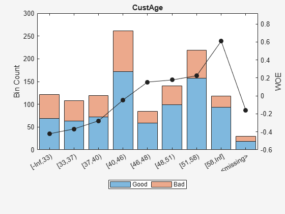
Display and plot bin information for categorical data for 'ResStatus' that includes missing data in a separate bin labelled <missing>.
[bi,cg] = bininfo(sc,'ResStatus');
disp(bi) Bin Good Bad Odds WOE InfoValue
______________ ____ ___ ______ _________ __________
{'Tenant' } 296 161 1.8385 -0.095463 0.0035249
{'Home Owner'} 352 171 2.0585 0.017549 0.00013382
{'Other' } 128 52 2.4615 0.19637 0.0055808
{'<missing>' } 27 13 2.0769 0.026469 2.3248e-05
{'Totals' } 803 397 2.0227 NaN 0.0092627
plotbins(sc,'ResStatus')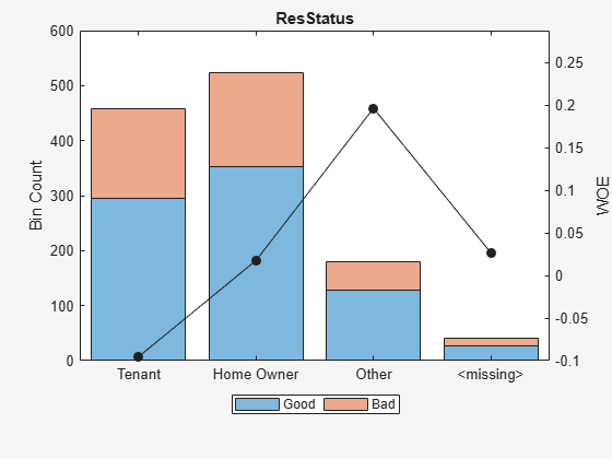
For the 'CustAge' and 'ResStatus' predictors, there is missing data (NaNs and <undefined>) in the training data, and the binning process estimates a WOE value of -0.15787 and 0.026469 respectively for missing data in these predictors, as shown above.
Use fitmodel to fit a logistic regression model using Weight of Evidence (WOE) data. fitmodel internally transforms all the predictor variables into WOE values, using the bins found with the automatic binning process. fitmodel then fits a logistic regression model using a stepwise method (by default). For predictors that have missing data, there is an explicit <missing> bin, with a corresponding WOE value computed from the data. When using fitmodel, the corresponding WOE value for the <missing> bin is applied when performing the WOE transformation.
[sc,mdl] = fitmodel(sc);
1. Adding CustIncome, Deviance = 1490.8527, Chi2Stat = 32.588614, PValue = 1.1387992e-08
2. Adding TmWBank, Deviance = 1467.1415, Chi2Stat = 23.711203, PValue = 1.1192909e-06
3. Adding AMBalance, Deviance = 1455.5715, Chi2Stat = 11.569967, PValue = 0.00067025601
4. Adding EmpStatus, Deviance = 1447.3451, Chi2Stat = 8.2264038, PValue = 0.0041285257
5. Adding CustAge, Deviance = 1442.8477, Chi2Stat = 4.4974731, PValue = 0.033944979
6. Adding ResStatus, Deviance = 1438.9783, Chi2Stat = 3.86941, PValue = 0.049173805
7. Adding OtherCC, Deviance = 1434.9751, Chi2Stat = 4.0031966, PValue = 0.045414057
Generalized linear regression model:
logit(status) ~ 1 + CustAge + ResStatus + EmpStatus + CustIncome + TmWBank + OtherCC + AMBalance
Distribution = Binomial
Estimated Coefficients:
Estimate SE tStat pValue
________ ________ ______ __________
(Intercept) 0.70229 0.063959 10.98 4.7498e-28
CustAge 0.57421 0.25708 2.2335 0.025513
ResStatus 1.3629 0.66952 2.0356 0.04179
EmpStatus 0.88373 0.2929 3.0172 0.002551
CustIncome 0.73535 0.2159 3.406 0.00065929
TmWBank 1.1065 0.23267 4.7556 1.9783e-06
OtherCC 1.0648 0.52826 2.0156 0.043841
AMBalance 1.0446 0.32197 3.2443 0.0011775
1200 observations, 1192 error degrees of freedom
Dispersion: 1
Chi^2-statistic vs. constant model: 88.5, p-value = 2.55e-16
Display unscaled points for predictors retained in the fitting model (to scale points use formatpoints).
PointsInfo = displaypoints(sc)
PointsInfo=38×3 table
Predictors Bin Points
_____________ ______________ _________
{'CustAge' } {'[-Inf,33)' } -0.14173
{'CustAge' } {'[33,37)' } -0.11095
{'CustAge' } {'[37,40)' } -0.059244
{'CustAge' } {'[40,46)' } 0.074167
{'CustAge' } {'[46,48)' } 0.1889
{'CustAge' } {'[48,51)' } 0.20204
{'CustAge' } {'[51,58)' } 0.22935
{'CustAge' } {'[58,Inf]' } 0.45019
{'CustAge' } {'<missing>' } 0.0096749
{'ResStatus'} {'Tenant' } -0.029778
{'ResStatus'} {'Home Owner'} 0.12425
{'ResStatus'} {'Other' } 0.36796
{'ResStatus'} {'<missing>' } 0.1364
{'EmpStatus'} {'Unknown' } -0.075948
{'EmpStatus'} {'Employed' } 0.31401
{'EmpStatus'} {'<missing>' } NaN
⋮
Notice that points for the <missing> bin for CustAge and ResStatus are explicitly shown. These points are computed from the WOE value for the <missing> bin and the logistic model coefficients.
For predictors that have no missing data in the training set, there is no explicit <missing> bin, and by default the points are set to NaN for missing data, and they lead to a score of NaN when running score. For predictors that have no explicit <missing> bin, use the name-value argument 'Missing' in formatpoints to indicate how missing data should be treated for scoring purposes.
This example shows how to use formatpoints after a model is fitted to format scaled points, and then use displaypoints to display the scaled points per bin, for a given predictor in the creditscorecard model.
Points become scaled when a range is defined. Specifically, a linear transformation from the unscaled to the scaled points is necessary. This transformation is defined either by supplying a shift and slope or by specifying the worst and best scores possible. (For more information, see formatpoints.)
Create a creditscorecard object using the CreditCardData.mat file to load the data (using a dataset from Refaat 2011). Use the 'IDVar' argument in the creditscorecard function to indicate that 'CustID' contains ID information and should not be included as a predictor variable.
load CreditCardData sc = creditscorecard(data,'IDVar','CustID');
Perform automatic binning to bin for all predictors.
sc = autobinning(sc);
Fit a linear regression model using default parameters.
sc = fitmodel(sc);
1. Adding CustIncome, Deviance = 1490.8527, Chi2Stat = 32.588614, PValue = 1.1387992e-08
2. Adding TmWBank, Deviance = 1467.1415, Chi2Stat = 23.711203, PValue = 1.1192909e-06
3. Adding AMBalance, Deviance = 1455.5715, Chi2Stat = 11.569967, PValue = 0.00067025601
4. Adding EmpStatus, Deviance = 1447.3451, Chi2Stat = 8.2264038, PValue = 0.0041285257
5. Adding CustAge, Deviance = 1441.994, Chi2Stat = 5.3511754, PValue = 0.020708306
6. Adding ResStatus, Deviance = 1437.8756, Chi2Stat = 4.118404, PValue = 0.042419078
7. Adding OtherCC, Deviance = 1433.707, Chi2Stat = 4.1686018, PValue = 0.041179769
Generalized linear regression model:
logit(status) ~ 1 + CustAge + ResStatus + EmpStatus + CustIncome + TmWBank + OtherCC + AMBalance
Distribution = Binomial
Estimated Coefficients:
Estimate SE tStat pValue
________ ________ ______ __________
(Intercept) 0.70239 0.064001 10.975 5.0538e-28
CustAge 0.60833 0.24932 2.44 0.014687
ResStatus 1.377 0.65272 2.1097 0.034888
EmpStatus 0.88565 0.293 3.0227 0.0025055
CustIncome 0.70164 0.21844 3.2121 0.0013179
TmWBank 1.1074 0.23271 4.7589 1.9464e-06
OtherCC 1.0883 0.52912 2.0569 0.039696
AMBalance 1.045 0.32214 3.2439 0.0011792
1200 observations, 1192 error degrees of freedom
Dispersion: 1
Chi^2-statistic vs. constant model: 89.7, p-value = 1.4e-16
Use the formatpoints function to scale providing the 'Worst' and 'Best' score values. The range provided below is a common score range.
sc = formatpoints(sc,'WorstAndBestScores',[300 850]);Display the points information again to verify that the points are now scaled and also display the scaled minimum and maximum scores.
[PointsInfo,MinScore,MaxScore]
= displaypoints(sc)
PointsInfo=37×3 table
Predictors Bin Points
______________ ________________ ______
{'CustAge' } {'[-Inf,33)' } 46.396
{'CustAge' } {'[33,37)' } 48.727
{'CustAge' } {'[37,40)' } 58.772
{'CustAge' } {'[40,46)' } 72.167
{'CustAge' } {'[46,48)' } 93.256
{'CustAge' } {'[48,58)' } 95.256
{'CustAge' } {'[58,Inf]' } 126.46
{'CustAge' } {'<missing>' } NaN
{'ResStatus' } {'Tenant' } 62.421
{'ResStatus' } {'Home Owner' } 82.276
{'ResStatus' } {'Other' } 113.58
{'ResStatus' } {'<missing>' } NaN
{'EmpStatus' } {'Unknown' } 56.765
{'EmpStatus' } {'Employed' } 105.81
{'EmpStatus' } {'<missing>' } NaN
{'CustIncome'} {'[-Inf,29000)'} 8.9706
⋮
MinScore = 300.0000
MaxScore = 850.0000
Notice that, as expected, the values of MinScore and MaxScore correspond to the worst and best possible scores.
This example shows how to use displaypoints after a model is fitted to separate the base points from the rest of the points assigned to each predictor variable. The name-value pair argument 'BasePoints' in the formatpoints function is a boolean that serves this purpose. By default, the base points are spread across all variables in the scorecard.
Create a creditscorecard object using the CreditCardData.mat file to load the data (using a dataset from Refaat 2011). Use the 'IDVar' argument in the creditscorecard function to indicate that 'CustID' contains ID information and should not be included as a predictor variable.
load CreditCardData sc = creditscorecard(data,'IDVar','CustID');
Perform automatic binning to bin for all predictors.
sc = autobinning(sc);
Fit a linear regression model using default parameters.
sc = fitmodel(sc);
1. Adding CustIncome, Deviance = 1490.8527, Chi2Stat = 32.588614, PValue = 1.1387992e-08
2. Adding TmWBank, Deviance = 1467.1415, Chi2Stat = 23.711203, PValue = 1.1192909e-06
3. Adding AMBalance, Deviance = 1455.5715, Chi2Stat = 11.569967, PValue = 0.00067025601
4. Adding EmpStatus, Deviance = 1447.3451, Chi2Stat = 8.2264038, PValue = 0.0041285257
5. Adding CustAge, Deviance = 1441.994, Chi2Stat = 5.3511754, PValue = 0.020708306
6. Adding ResStatus, Deviance = 1437.8756, Chi2Stat = 4.118404, PValue = 0.042419078
7. Adding OtherCC, Deviance = 1433.707, Chi2Stat = 4.1686018, PValue = 0.041179769
Generalized linear regression model:
logit(status) ~ 1 + CustAge + ResStatus + EmpStatus + CustIncome + TmWBank + OtherCC + AMBalance
Distribution = Binomial
Estimated Coefficients:
Estimate SE tStat pValue
________ ________ ______ __________
(Intercept) 0.70239 0.064001 10.975 5.0538e-28
CustAge 0.60833 0.24932 2.44 0.014687
ResStatus 1.377 0.65272 2.1097 0.034888
EmpStatus 0.88565 0.293 3.0227 0.0025055
CustIncome 0.70164 0.21844 3.2121 0.0013179
TmWBank 1.1074 0.23271 4.7589 1.9464e-06
OtherCC 1.0883 0.52912 2.0569 0.039696
AMBalance 1.045 0.32214 3.2439 0.0011792
1200 observations, 1192 error degrees of freedom
Dispersion: 1
Chi^2-statistic vs. constant model: 89.7, p-value = 1.4e-16
Use the formatpoints function to separate the base points by providing the 'BasePoints' name-value pair argument.
sc = formatpoints(sc,'BasePoints',true);Display the base points, separated out from the other points, for predictors retained in the fitting model.
PointsInfo = displaypoints(sc)
PointsInfo=38×3 table
Predictors Bin Points
______________ ______________ _________
{'BasePoints'} {'BasePoints'} 0.70239
{'CustAge' } {'[-Inf,33)' } -0.25928
{'CustAge' } {'[33,37)' } -0.24071
{'CustAge' } {'[37,40)' } -0.16066
{'CustAge' } {'[40,46)' } -0.053933
{'CustAge' } {'[46,48)' } 0.11411
{'CustAge' } {'[48,58)' } 0.13005
{'CustAge' } {'[58,Inf]' } 0.37866
{'CustAge' } {'<missing>' } NaN
{'ResStatus' } {'Tenant' } -0.13159
{'ResStatus' } {'Home Owner'} 0.026616
{'ResStatus' } {'Other' } 0.27607
{'ResStatus' } {'<missing>' } NaN
{'EmpStatus' } {'Unknown' } -0.17666
{'EmpStatus' } {'Employed' } 0.21415
{'EmpStatus' } {'<missing>' } NaN
⋮
This example shows how to use displaypoints after a model is fitted and the modifybins function is used to provide user-defined bin labels for a numeric predictor.
Create a creditscorecard object using the CreditCardData.mat file to load the data (using a dataset from Refaat 2011). Use the 'IDVar' argument in the creditscorecard function to indicate that 'CustID' contains ID information and should not be included as a predictor variable.
load CreditCardData sc = creditscorecard(data,'IDVar','CustID');
Perform automatic binning to bin for all predictors.
sc = autobinning(sc);
Fit a linear regression model using default parameters.
sc = fitmodel(sc);
1. Adding CustIncome, Deviance = 1490.8527, Chi2Stat = 32.588614, PValue = 1.1387992e-08
2. Adding TmWBank, Deviance = 1467.1415, Chi2Stat = 23.711203, PValue = 1.1192909e-06
3. Adding AMBalance, Deviance = 1455.5715, Chi2Stat = 11.569967, PValue = 0.00067025601
4. Adding EmpStatus, Deviance = 1447.3451, Chi2Stat = 8.2264038, PValue = 0.0041285257
5. Adding CustAge, Deviance = 1441.994, Chi2Stat = 5.3511754, PValue = 0.020708306
6. Adding ResStatus, Deviance = 1437.8756, Chi2Stat = 4.118404, PValue = 0.042419078
7. Adding OtherCC, Deviance = 1433.707, Chi2Stat = 4.1686018, PValue = 0.041179769
Generalized linear regression model:
logit(status) ~ 1 + CustAge + ResStatus + EmpStatus + CustIncome + TmWBank + OtherCC + AMBalance
Distribution = Binomial
Estimated Coefficients:
Estimate SE tStat pValue
________ ________ ______ __________
(Intercept) 0.70239 0.064001 10.975 5.0538e-28
CustAge 0.60833 0.24932 2.44 0.014687
ResStatus 1.377 0.65272 2.1097 0.034888
EmpStatus 0.88565 0.293 3.0227 0.0025055
CustIncome 0.70164 0.21844 3.2121 0.0013179
TmWBank 1.1074 0.23271 4.7589 1.9464e-06
OtherCC 1.0883 0.52912 2.0569 0.039696
AMBalance 1.045 0.32214 3.2439 0.0011792
1200 observations, 1192 error degrees of freedom
Dispersion: 1
Chi^2-statistic vs. constant model: 89.7, p-value = 1.4e-16
Use the displaypoints function to display point information.
[PointsInfo,MinScore,MaxScore]
= displaypoints(sc)
PointsInfo=37×3 table
Predictors Bin Points
______________ ________________ _________
{'CustAge' } {'[-Inf,33)' } -0.15894
{'CustAge' } {'[33,37)' } -0.14036
{'CustAge' } {'[37,40)' } -0.060323
{'CustAge' } {'[40,46)' } 0.046408
{'CustAge' } {'[46,48)' } 0.21445
{'CustAge' } {'[48,58)' } 0.23039
{'CustAge' } {'[58,Inf]' } 0.479
{'CustAge' } {'<missing>' } NaN
{'ResStatus' } {'Tenant' } -0.031252
{'ResStatus' } {'Home Owner' } 0.12696
{'ResStatus' } {'Other' } 0.37641
{'ResStatus' } {'<missing>' } NaN
{'EmpStatus' } {'Unknown' } -0.076317
{'EmpStatus' } {'Employed' } 0.31449
{'EmpStatus' } {'<missing>' } NaN
{'CustIncome'} {'[-Inf,29000)'} -0.45716
⋮
MinScore = -1.3100
MaxScore = 3.0726
Use the modifybins function to specify user-defined bin labels for 'CustAge' so that the bin ranges are described in natural language.
labels = {'Up to 32','33 to 36','37 to 39','40 to 45','46 to 47','48 to 57','At least 58'};
sc = modifybins(sc,'CustAge','BinLabels',labels);Rerun displaypoints to verify the updated bin labels.
[PointsInfo,MinScore,MaxScore] = displaypoints(sc)
PointsInfo=37×3 table
Predictors Bin Points
______________ ________________ _________
{'CustAge' } {'Up to 32' } -0.15894
{'CustAge' } {'33 to 36' } -0.14036
{'CustAge' } {'37 to 39' } -0.060323
{'CustAge' } {'40 to 45' } 0.046408
{'CustAge' } {'46 to 47' } 0.21445
{'CustAge' } {'48 to 57' } 0.23039
{'CustAge' } {'At least 58' } 0.479
{'CustAge' } {'<missing>' } NaN
{'ResStatus' } {'Tenant' } -0.031252
{'ResStatus' } {'Home Owner' } 0.12696
{'ResStatus' } {'Other' } 0.37641
{'ResStatus' } {'<missing>' } NaN
{'EmpStatus' } {'Unknown' } -0.076317
{'EmpStatus' } {'Employed' } 0.31449
{'EmpStatus' } {'<missing>' } NaN
{'CustIncome'} {'[-Inf,29000)'} -0.45716
⋮
MinScore = -1.3100
MaxScore = 3.0726
This example shows how to use a credit scorecard to compute the weights of the predictors. The weights of the predictors are determined from the range of points of each predictor, divided by the total range of points for the scorecard. The points for the scorecard not only take into consideration the betas, but also implicitly the binning of the predictor values and the corresponding weights of evidence.
Create a scorecard.
load CreditCardData.mat sc = creditscorecard(data,'IDVar','CustID'); sc = autobinning(sc); sc = fitmodel(sc);
1. Adding CustIncome, Deviance = 1490.8527, Chi2Stat = 32.588614, PValue = 1.1387992e-08
2. Adding TmWBank, Deviance = 1467.1415, Chi2Stat = 23.711203, PValue = 1.1192909e-06
3. Adding AMBalance, Deviance = 1455.5715, Chi2Stat = 11.569967, PValue = 0.00067025601
4. Adding EmpStatus, Deviance = 1447.3451, Chi2Stat = 8.2264038, PValue = 0.0041285257
5. Adding CustAge, Deviance = 1441.994, Chi2Stat = 5.3511754, PValue = 0.020708306
6. Adding ResStatus, Deviance = 1437.8756, Chi2Stat = 4.118404, PValue = 0.042419078
7. Adding OtherCC, Deviance = 1433.707, Chi2Stat = 4.1686018, PValue = 0.041179769

Generalized linear regression model:
    logit(status) ~ 1 + CustAge + ResStatus + EmpStatus + CustIncome + TmWBank + OtherCC + AMBalance
    Distribution = Binomial

Estimated Coefficients:
                   Estimate       SE       tStat       pValue
                   ________    ________    ______    __________

    (Intercept)    0.70239     0.064001    10.975    5.0538e-28
    CustAge        0.60833      0.24932      2.44      0.014687
    ResStatus        1.377      0.65272    2.1097      0.034888
    EmpStatus      0.88565        0.293    3.0227     0.0025055
    CustIncome     0.70164      0.21844    3.2121     0.0013179
    TmWBank         1.1074      0.23271    4.7589    1.9464e-06
    OtherCC         1.0883      0.52912    2.0569      0.039696
    AMBalance        1.045      0.32214    3.2439     0.0011792


1200 observations, 1192 error degrees of freedom
Dispersion: 1
Chi^2-statistic vs. constant model: 89.7, p-value = 1.4e-16
Compute scorecard points and the MinPts and MaxPts scores.
sc = formatpoints(sc,'PointsOddsAndPDO',[500 2 50]);
[PointsTable,MinPts,MaxPts] = displaypoints(sc);
PtsRange = MaxPts-MinPts;
disp(PointsTable(1:10,:)); Predictors Bin Points
_____________ ______________ ______
{'CustAge' } {'[-Inf,33)' } 52.821
{'CustAge' } {'[33,37)' } 54.161
{'CustAge' } {'[37,40)' } 59.934
{'CustAge' } {'[40,46)' } 67.633
{'CustAge' } {'[46,48)' } 79.755
{'CustAge' } {'[48,58)' } 80.905
{'CustAge' } {'[58,Inf]' } 98.838
{'CustAge' } {'<missing>' } NaN
{'ResStatus'} {'Tenant' } 62.031
{'ResStatus'} {'Home Owner'} 73.444
fprintf('Min points: %g, Max points: %g\n',MinPts,MaxPts); Min points: 355.505, Max points: 671.64
Compute the predictor weights.
Predictor = unique(PointsTable.Predictors,'stable'); NumPred = length(Predictor); Weight = zeros(NumPred,1); for ii=1:NumPred Ind = cellfun(@(x)strcmpi(Predictor{ii},x),PointsTable.Predictors); MaxPtsPred = max(PointsTable.Points(Ind)); MinPtsPred = min(PointsTable.Points(Ind)); Weight(ii) = 100*(MaxPtsPred-MinPtsPred)/PtsRange; end PredictorWeights = table(Predictor,Weight); PredictorWeights(end+1,:) = PredictorWeights(end,:); PredictorWeights.Predictor{end} = 'Total'; PredictorWeights.Weight(end) = sum(Weight); disp(PredictorWeights)
Predictor Weight
______________ ______
{'CustAge' } 14.556
{'ResStatus' } 9.302
{'EmpStatus' } 8.9174
{'CustIncome'} 20.401
{'TmWBank' } 25.884
{'OtherCC' } 7.9885
{'AMBalance' } 12.951
{'Total' } 100
The weights are defined as the range of points for the predictor divided by the range of points for the scorecard.
To create a creditscorecard object using the CreditCardData.mat file, load the data (using a dataset from Refaat 2011). Using the dataMissing dataset, set the 'BinMissingData' indicator to true.
load CreditCardData.mat sc = creditscorecard(dataMissing,'BinMissingData',true);
Use autobinning with the creditscorecard object.
sc = autobinning(sc);
The binning map or rules for categorical data are summarized in a "category grouping" table, returned as an optional output. By default, each category is placed in a separate bin. Here is the information for the predictor ResStatus.
[bi,cg] = bininfo(sc,'ResStatus')bi=5×6 table
         Bin          Good    Bad     Odds        WOE       InfoValue
    ______________    ____    ___    ______    _________    __________

    {'Tenant'    }    296     161    1.8385    -0.095463     0.0035249
    {'Home Owner'}    352     171    2.0585     0.017549    0.00013382
    {'Other'     }    128      52    2.4615      0.19637     0.0055808
    {'<missing>' }     27      13    2.0769     0.026469    2.3248e-05
    {'Totals'    }    803     397    2.0227          NaN     0.0092627
cg=3×2 table
Category BinNumber
______________ _________
{'Tenant' } 1
{'Home Owner'} 2
{'Other' } 3
To group categories 'Tenant' and 'Other', modify the category grouping table cg, so the bin number for 'Other' is the same as the bin number for 'Tenant'. Then use modifybins to update the creditscorecard object.
cg.BinNumber(3) = 2; sc = modifybins(sc,'ResStatus','Catg',cg);
Display the updated bin information using bininfo. Note that the bin labels has been updated and that the bin membership information is contained in the category grouping cg.
[bi,cg] = bininfo(sc,'ResStatus')bi=4×6 table
Bin Good Bad Odds WOE InfoValue
_____________ ____ ___ ______ _________ __________
{'Group1' } 296 161 1.8385 -0.095463 0.0035249
{'Group2' } 480 223 2.1525 0.062196 0.0022419
{'<missing>'} 27 13 2.0769 0.026469 2.3248e-05
{'Totals' } 803 397 2.0227 NaN 0.00579
cg=3×2 table
Category BinNumber
______________ _________
{'Tenant' } 1
{'Home Owner'} 2
{'Other' } 2
Use formatpoints with the 'Missing' name-value pair argument to indicate that missing data is assigned 'maxpoints'.
sc = formatpoints(sc,'BasePoints',true,'Missing','maxpoints','WorstAndBest',[300 800]);
Use fitmodel to fit the model.
sc = fitmodel(sc,'VariableSelection','fullmodel','Display','Off');
Then use displaypoints (Risk Management Toolbox) with the creditscorecard object to return a table of points for all bins of all predictor variables used in the compactCreditScorecard object. By setting the displaypoints (Risk Management Toolbox) name-value pair argument for 'ShowCategoricalMembers' to true, all the members contained in each individual group are displayed.
[PointsInfo,MinScore,MaxScore] = displaypoints(sc,'ShowCategoricalMembers',true)PointsInfo=51×3 table
Predictors Bin Points
_______________ ______________ _______
{'BasePoints' } {'BasePoints'} 535.25
{'CustID' } {'[-Inf,121)'} 12.085
{'CustID' } {'[121,241)' } 5.4738
{'CustID' } {'[241,1081)'} -1.4061
{'CustID' } {'[1081,Inf]'} -7.2217
{'CustID' } {'<missing>' } 12.085
{'CustAge' } {'[-Inf,33)' } -25.973
{'CustAge' } {'[33,37)' } -22.67
{'CustAge' } {'[37,40)' } -17.122
{'CustAge' } {'[40,46)' } -2.8071
{'CustAge' } {'[46,48)' } 9.5034
{'CustAge' } {'[48,51)' } 10.913
{'CustAge' } {'[51,58)' } 13.844
{'CustAge' } {'[58,Inf]' } 37.541
{'CustAge' } {'<missing>' } -9.7271
{'TmAtAddress'} {'[-Inf,23)' } -9.3683
⋮
MinScore =
300.0000
MaxScore =
800
Input Arguments
Name-Value Arguments
Output Arguments
Algorithms
The points for predictor j and bin i are, by default, given by
Points_ji = (Shift + Slope*b0)/p + Slope*(bj*WOEj(i))
Shift and Slope are scaling constants.When the base points are reported separately (see the formatpoints name-value pair argument BasePoints),
the base points are given
by
Base Points = Shift + Slope*b0,
Points_ji = Slope*(bj*WOEj(i))).
By default, the base points are not reported separately.
The minimum and maximum scores are:
MinScore = Shift + Slope*b0 + min(Slope*b1*WOE1) + ... +min(Slope*bp*WOEp)),
MaxScore = Shift + Slope*b0 + max(Slope*b1*WOE1) + ... +max(Slope*bp*WOEp)).
Use formatpoints to control the way points
are scaled, rounded, and whether the base points are reported separately. See formatpoints for more information on format parameters and for details
and formulas on these formatting options.
References
[1] Anderson, R. The Credit Scoring Toolkit. Oxford University Press, 2007.
[2] Refaat, M. Credit Risk Scorecards: Development and Implementation Using SAS. lulu.com, 2011.
Version History
Introduced in R2014b
See Also
creditscorecard | autobinning | bininfo | predictorinfo | modifypredictor | plotbins | fillmissing | modifybins | bindata | fitmodel | formatpoints | score | setmodel | probdefault | validatemodel