Main Content

fitsemigraph

Label data using semi-supervised graph-based method

Since R2020b

    Description

    fitsemigraph creates a semi-supervised graph-based model given labeled data, labels, and unlabeled data. The returned model contains the fitted labels for the unlabeled data and the corresponding scores. This model can also predict labels for unseen data using the predict object function. For more information on the different labeling algorithms, see Algorithms.

    example

    Mdl = fitsemigraph(Tbl,ResponseVarName,UnlabeledTbl) uses the labeled data in Tbl, where Tbl.ResponseVarName contains the labels for the labeled data, and returns fitted labels for the unlabeled data in UnlabeledTbl. The function stores the fitted labels and the corresponding scores in the FittedLabels and LabelScores properties of the object Mdl, respectively.

    Mdl = fitsemigraph(Tbl,formula,UnlabeledTbl) uses formula to specify the response variable (vector of labels) and the predictor variables to use among the variables in Tbl. The function uses these variables to label the data in UnlabeledTbl.

    Mdl = fitsemigraph(Tbl,Y,UnlabeledTbl) uses the predictor data in Tbl and the labels in Y to label the data in UnlabeledTbl.

    example

    Mdl = fitsemigraph(X,Y,UnlabeledX) uses the predictor data in X and the labels in Y to label the data in UnlabeledX.

    example

    Mdl = fitsemigraph(___,Name,Value) specifies options using one or more name-value pair arguments in addition to any of the input argument combinations in previous syntaxes. For example, you can specify the labeling method, number of iterations, and score threshold to use in the labeling algorithm.

    Examples

    collapse all

    Fit labels to unlabeled data by using a semi-supervised graph-based method.

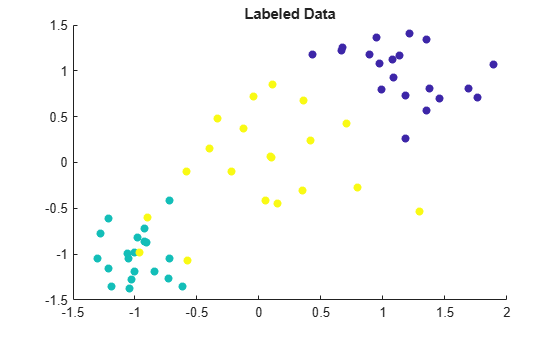
    Randomly generate 60 observations of labeled data, with 20 observations in each of three classes.

    rng('default') % For reproducibility
    
    labeledX = [randn(20,2)*0.25 + ones(20,2);
                randn(20,2)*0.25 - ones(20,2);
                randn(20,2)*0.5];
    Y = [ones(20,1); ones(20,1)*2; ones(20,1)*3];

    Visualize the labeled data by using a scatter plot. Observations in the same class have the same color. Notice that the data is split into three clusters with very little overlap.

    scatter(labeledX(:,1),labeledX(:,2),[],Y,'filled')
    title('Labeled Data')

    Figure contains an axes object. The axes object with title Labeled Data contains an object of type scatter.

    Randomly generate 300 additional observations of unlabeled data, with 100 observations per class. For the purposes of validation, keep track of the true labels for the unlabeled data.

    unlabeledX = [randn(100,2)*0.25 + ones(100,2);
                  randn(100,2)*0.25 - ones(100,2);
                  randn(100,2)*0.5];
    trueLabels = [ones(100,1); ones(100,1)*2; ones(100,1)*3];

    Fit labels to the unlabeled data by using a semi-supervised graph-based method. The function fitsemigraph returns a SemiSupervisedGraphModel object whose FittedLabels property contains the fitted labels for the unlabeled data and whose LabelScores property contains the associated label scores.

    Mdl = fitsemigraph(labeledX,Y,unlabeledX)
    Mdl = 
      SemiSupervisedGraphModel with properties:
    
                 FittedLabels: [300x1 double]
                  LabelScores: [300x3 double]
                   ClassNames: [1 2 3]
                 ResponseName: 'Y'
        CategoricalPredictors: []
                       Method: 'labelpropagation'


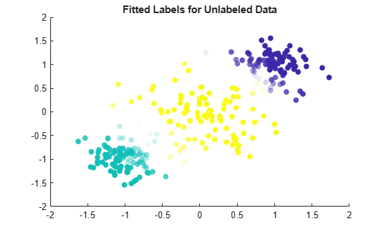
    Visualize the fitted label results by using a scatter plot. Use the fitted labels to set the color of the observations, and use the maximum label scores to set the transparency of the observations. Observations with less transparency are labeled with greater confidence. Notice that observations that lie closer to the cluster boundaries are labeled with more uncertainty.

    maxLabelScores = max(Mdl.LabelScores,[],2);
    rescaledScores = rescale(maxLabelScores,0.05,0.95);
    scatter(unlabeledX(:,1),unlabeledX(:,2),[],Mdl.FittedLabels,'filled', ...
        'MarkerFaceAlpha','flat','AlphaData',rescaledScores);
    title('Fitted Labels for Unlabeled Data')

    Figure contains an axes object. The axes object with title Fitted Labels for Unlabeled Data contains an object of type scatter.

    Determine the accuracy of the labeling by using the true labels for the unlabeled data.

    numWrongLabels = sum(trueLabels ~= Mdl.FittedLabels)
    numWrongLabels = 10
    

    Only 10 of the 300 observations in unlabeledX are mislabeled.

    Fit labels to unlabeled data by using a semi-supervised graph-based method. Specify the type of nearest neighbor graph.

    Load the patients data set. Create a table from the variables Distolic, Gender, and so on. For each observation, or row in the table, treat the Smoker value as the label for that observation.

    load patients
    Tbl = table(Diastolic,Gender,Height,Systolic,Weight,Smoker);

    Suppose only 20% of the observations are labeled. To recreate this scenario, randomly sample 20 labeled observations and store them in the table unlabeledTbl. Remove the label from the rest of the observations and store them in the table unlabeledTbl. To verify the accuracy of the label fitting at the end of the example, retain the true labels for the unlabeled data in the variable trueLabels.

    rng('default') % For reproducibility of the sampling
    [labeledTbl,Idx] = datasample(Tbl,20,'Replace',false);
    
    unlabeledTbl = Tbl;
    unlabeledTbl(Idx,:) = [];
    trueLabels = unlabeledTbl.Smoker;
    unlabeledTbl.Smoker = [];

    Fit labels to the unlabeled data by using a semi-supervised graph-based method. Use a mutual type of nearest neighbor graph, where two points are connected when they are nearest neighbors of each other. Specify to standardize the numeric predictors. The function fitsemigraph returns an object whose FittedLabels property contains the fitted labels for the unlabeled data.

    Mdl = fitsemigraph(labeledTbl,'Smoker',unlabeledTbl,'KNNGraphType','mutual', ...
        'Standardize',true);
    fittedLabels = Mdl.FittedLabels;

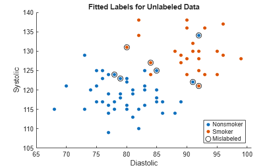
    Identify the observations that are incorrectly labeled by comparing the stored true labels for the unlabeled data to the fitted labels returned by the semi-supervised graph-based method.

    wrongIdx = (trueLabels ~= fittedLabels);
    wrongTbl = unlabeledTbl(wrongIdx,:);

    Visualize the fitted label results for the unlabeled data. Mislabeled observations are circled in the plot.

    gscatter(unlabeledTbl.Diastolic,unlabeledTbl.Systolic, ...
        fittedLabels)
    hold on
    plot(wrongTbl.Diastolic,wrongTbl.Systolic, ...
        'ko','MarkerSize',8)
    xlabel('Diastolic')
    ylabel('Systolic')
    legend('Nonsmoker','Smoker','Mislabeled')
    title('Fitted Labels for Unlabeled Data')

    Figure contains an axes object. The axes object with title Fitted Labels for Unlabeled Data, xlabel Diastolic, ylabel Systolic contains 3 objects of type line. One or more of the lines displays its values using only markers These objects represent Nonsmoker, Smoker, Mislabeled.

    Input Arguments

    collapse all

    Labeled sample data, specified as a table. Each row of Tbl corresponds to one observation, and each column corresponds to one predictor. Optionally, Tbl can contain one additional column for the response variable (vector of labels). Multicolumn variables, cell arrays other than cell arrays of character vectors, and ordinal categorical variables are not supported.

    If Tbl contains the response variable, and you want to use all remaining variables in Tbl as predictors, then specify the response variable using ResponseVarName.

    If Tbl contains the response variable, and you want to use only a subset of the remaining variables in Tbl as predictors, specify a formula using formula.

    If Tbl does not contain the response variable, specify a response variable using Y. The length of the response variable and the number of rows in Tbl must be equal.

    Data Types: table

    Unlabeled sample data, specified as a table. Each row of UnlabeledTbl corresponds to one observation, and each column corresponds to one predictor. UnlabeledTbl must contain the same predictors as those contained in Tbl.

    Data Types: table

    Response variable name, specified as the name of a variable in Tbl. The response variable contains the class labels for the sample data in Tbl.

    You must specify ResponseVarName as a character vector or string scalar. For example, if the response variable Y is stored as Tbl.Y, then specify it as 'Y'. Otherwise, the software treats all columns of Tbl, including Y, as predictors.

    The response variable must be a categorical, character, or string array, a logical or numeric vector, or a cell array of character vectors. If Y is a character array, then each element of the response variable must correspond to one row of the array.

    A good practice is to specify the order of the classes by using the ClassNames name-value pair argument.

    Data Types: char | string

    Explanatory model of the response variable and a subset of the predictor variables, specified as a character vector or string scalar in the form 'Y~X1+X2+X3'. In this form, Y represents the response variable, and X1, X2, and X3 represent the predictor variables.

    To specify a subset of variables in Tbl as predictors, use a formula. If you specify a formula, then the software does not use any variables in Tbl that do not appear in formula.

    The variable names in the formula must be both variable names in Tbl (Tbl.Properties.VariableNames) and valid MATLAB® identifiers. You can verify the variable names in Tbl by using the isvarname function. If the variable names are not valid, then you can convert them by using the matlab.lang.makeValidName function.

    Data Types: char | string

    Class labels, specified as a numeric, categorical, or logical vector, a character or string array, or a cell array of character vectors.

    • If Y is a character array, then each element of the class labels must correspond to one row of the array.

    • The length of Y must be equal to the number of rows in Tbl or X.

    • A good practice is to specify the class order by using the ClassNames name-value pair argument.

    Data Types: single | double | categorical | logical | char | string | cell

    Labeled predictor data, specified as a numeric matrix.

    Each row of X corresponds to one observation, and each column corresponds to one predictor.

    The length of Y and the number of rows in X must be equal.

    To specify the names of the predictors in the order of their appearance in X, use the PredictorNames name-value pair argument.

    Data Types: single | double

    Unlabeled predictor data, specified as a numeric matrix. Each row of UnlabeledX corresponds to one observation, and each column corresponds to one predictor. UnlabeledX must have the same predictors as X, in the same order.

    Data Types: single | double

    Note

    The software treats NaN, empty character vector (''), empty string (""), <missing>, and <undefined> elements as missing data. The software removes rows of the predictor data (observations) with missing values.

    Name-Value Arguments

    Specify optional pairs of arguments as Name1=Value1,...,NameN=ValueN, where Name is the argument name and Value is the corresponding value. Name-value arguments must appear after other arguments, but the order of the pairs does not matter.

    Before R2021a, use commas to separate each name and value, and enclose Name in quotes.

    Example: fitsemigraph(Tbl,'Y',UnlabeledTbl,'Method','labelspreading','IterationLimit',2e3) specifies to use a label spreading labeling technique and run a maximum of 2000 iterations.

    Labeling Algorithm Options

    collapse all

    Labeling technique, specified as the comma-separated pair consisting of 'Method' and one of these values.

    ValueDescriptionMethod-Specific Name-Value Pair Arguments
    'labelpropagation'Iteratively propagate labels across the nodes in the similarity graph. For more information, see Label Propagation.

    'IterationLimit' — Maximum number of iterations

    'Tolerance' — Tolerance for the score absolute difference in subsequent iterations

    'labelpropagationexact'Use an exact formula to propagate labels. For more information, see Label Propagation.None
    'labelspreading'Iteratively spread labels across the nodes in the similarity graph. For more information, see Label Spreading.

    'Alpha' — Relative weight of neighboring labels to the initial label

    'IterationLimit' — Maximum number of iterations

    'Tolerance' — Tolerance for the score absolute difference in subsequent iterations

    'labelspreadingexact'Use an exact formula to spread labels. For more information, see Label Spreading.

    'Alpha' — Relative weight of neighboring labels to the initial label

    Example: 'Method','labelspreading'

    Data Types: char | string

    Relative weight of neighboring labels to the initial label for labeled observations in X or Tbl, specified as the comma-separated pair consisting of 'Alpha' and a scalar value in the range (0,1). A value close to 0 indicates that fitsemigraph treats labels of initially labeled observations almost like ground truth. A value close to 1 indicates that fitsemigraph treats labels of initially labeled observations almost like noise.

    Note

    This argument is valid only when the Method value is 'labelspreading' or 'labelspreadingexact'.

    Example: 'Alpha',0.05

    Data Types: single | double

    Maximum number of iterations, specified as the comma-separated pair consisting of 'IterationLimit' and a positive integer scalar. The fitsemigraph function returns Mdl, which contains the fitted labels and scores, when this limit is reached, even if the algorithm does not converge.

    Note

    This argument is valid only when the Method value is 'labelpropagation' or 'labelspreading'.

    Example: 'IterationLimit',2e3

    Data Types: single | double

    Tolerance for score absolute difference in subsequent iterations, specified as the comma-separated pair consisting of 'Tolerance' and a nonnegative scalar.

    Note

    This argument is valid only when the Method value is 'labelpropagation' or 'labelspreading'.

    Example: 'Tolerance',1e-4

    Data Types: single | double

    Classification Options

    collapse all

    Categorical predictors list, specified as one of the values in this table.

    ValueDescription
    Vector of positive integers

    Each entry in the vector is an index value indicating that the corresponding predictor is categorical. The index values are between 1 and p, where p is the number of predictors used to train the model.

    If fitsemigraph uses a subset of input variables as predictors, then the function indexes the predictors using only the subset. The CategoricalPredictors values do not count the response variable, observation weights variable, or any other variables that the function does not use.

    Logical vector

    A true entry means that the corresponding predictor is categorical. The length of the vector is p.

    Character matrixEach row of the matrix is the name of a predictor variable. The names must match the entries in PredictorNames. Pad the names with extra blanks so each row of the character matrix has the same length.
    String array or cell array of character vectorsEach element in the array is the name of a predictor variable. The names must match the entries in PredictorNames.
    "all"All predictors are categorical.

    By default, if the predictor data is in a table, fitsemigraph assumes that a variable is categorical if it is a logical vector, categorical vector, character array, string array, or cell array of character vectors. Ordinal categorical variables are not supported. If the predictor data is a matrix, fitsemigraph assumes that all predictors are continuous. To identify any other predictors as categorical predictors, specify them by using the 'CategoricalPredictors' name-value pair argument.

    fitsemigraph encodes categorical variables as numeric variables by assigning a positive integer value to each category. When you use categorical predictors, ensure that you use an appropriate distance metric (Distance).

    Example: 'CategoricalPredictors','all'

    Data Types: single | double | logical | char | string | cell

    Names of the classes to use for labeling, specified as the comma-separated pair consisting of 'ClassNames' and a categorical, character, or string array, a logical or numeric vector, or a cell array of character vectors. ClassNames must have the same data type as Y.

    If ClassNames is a character array, then each element must correspond to one row of the array.

    Use 'ClassNames' to:

    • Order the classes.

    • Specify the order of any input or output argument dimension that corresponds to the class order. For example, use 'ClassNames' to specify the column order of classification scores in Mdl.LabelScores.

    • Select a subset of classes for labeling. For example, suppose that the set of all distinct class names in Y is {'a','b','c'}. To use observations from classes 'a' and 'c' only, specify 'ClassNames',{'a','c'}.

    The default value for ClassNames is the set of all distinct class names in Y.

    Example: 'ClassNames',{'b','g'}

    Data Types: categorical | char | string | logical | single | double | cell

    Predictor variable names, specified as the comma-separated pair consisting of 'PredictorNames' and a string array of unique names or cell array of unique character vectors. The functionality of 'PredictorNames' depends on the way you supply the predictor data.

    • If you supply X, Y, and UnlabeledX, then you can use 'PredictorNames' to assign names to the predictor variables in X and UnlabeledX.

      • The order of the names in PredictorNames must correspond to the column order of X. That is, PredictorNames{1} is the name of X(:,1), PredictorNames{2} is the name of X(:,2), and so on. Also, size(X,2) and numel(PredictorNames) must be equal.

      • By default, PredictorNames is {'x1','x2',...}.

    • If you supply Tbl and UnlabeledTbl, then you can use 'PredictorNames' to choose which predictor variables to use. That is, fitsemigraph uses only the predictor variables in PredictorNames and the response variable to label the unlabeled data.

      • PredictorNames must be a subset of Tbl.Properties.VariableNames and cannot include the name of the response variable.

      • By default, PredictorNames contains the names of all predictor variables.

      • A good practice is to specify the predictors using either 'PredictorNames' or formula, but not both.

    Example: 'PredictorNames',{'SepalLength','SepalWidth','PetalLength','PetalWidth'}

    Data Types: string | cell

    Response variable name, specified as the comma-separated pair consisting of 'ResponseName' and a character vector or string scalar.

    • If you supply Y, then you can use 'ResponseName' to specify a name for the response variable.

    • If you supply ResponseVarName or formula, then you cannot use 'ResponseName'.

    Example: 'ResponseName','response'

    Data Types: char | string

    Flag to standardize the predictor data, specified as the comma-separated pair consisting of 'Standardize' and a numeric or logical 0 (false) or 1 (true). If you set 'Standardize',true, the software combines the labeled and unlabeled predictor data, and then centers and scales each numeric predictor variable by the corresponding column mean and standard deviation. The software does not standardize the categorical predictors.

    Example: 'Standardize',true

    Data Types: double | logical

    Distance Metric Options

    collapse all

    Distance metric, specified as the comma-separated pair consisting of 'Distance' and a character vector or string scalar.

    • If all the predictor variables are continuous (numeric) variables, then you can specify one of these distance metrics.

      ValueDescription
      'euclidean'

      Euclidean distance

      'seuclidean'

      Standardized Euclidean distance — Each coordinate difference between observations is scaled by dividing by the corresponding element of the standard deviation S = std(PD,'omitnan'), where PD is the predictor data, both labeled and unlabeled. To specify another scale parameter, use the 'Scale' name-value pair argument.

      'mahalanobis'

      Mahalanobis distance — By default, the distance is computed using C = cov(PD,'omitrows'), the covariance of PD. To change the value of the covariance matrix, use the 'Cov' name-value pair argument.

      'minkowski'

      Minkowski distance — The default exponent is 2. To specify a different exponent, use the 'P' name-value pair argument.

      'chebychev'

      Chebychev distance (maximum coordinate difference)

      'cityblock'

      City block distance

      'correlation'

      One minus the sample correlation between observations (treated as sequences of values)

      'cosine'

      One minus the cosine of the included angle between observations (treated as vectors)

      'spearman'

      One minus the sample Spearman's rank correlation between observations (treated as sequences of values)

      Note

      If you specify one of these distance metrics and the predictor data includes categorical predictors, then the software treats each categorical predictor as a numeric variable for the distance computation, with each category represented by a positive integer. The Distance value does not affect the CategoricalPredictors property of the trained model.

    • If all the predictor variables are categorical variables, then you can specify one of these distance metrics.

      ValueDescription
      'hamming'

      Hamming distance, which is the percentage of coordinates that differ

      'jaccard'

      One minus the Jaccard coefficient, which is the percentage of nonzero coordinates that differ

      Note

      If you specify one of these distance metrics and the predictor data includes continuous (numeric) predictors, then the software treats each continuous predictor as a categorical variable for the distance computation. The Distance value does not affect the CategoricalPredictors property of the trained model.

    • If the predictor variables are a mix of continuous (numeric) and categorical variables, then you can specify one of these distance metrics.

      ValueDescription
      'goodall3'

      Modified Goodall distance

      'ofd'

      Occurrence frequency distance

    The default value is 'euclidean' if all the predictor variables are continuous, and 'goodall3' if any of the predictor variables are categorical. For more information on the various distance metrics, see Distance Metrics.

    Example: 'Distance','ofd'

    Data Types: char | string

    Scale parameter for the standardized Euclidean distance metric, specified as the comma-separated pair consisting of 'Scale' and a nonnegative vector. The length of Scale is equal to the number of predictors. Each coordinate difference between two observations is scaled by the corresponding element of Scale.

    The default scale parameter is std(PD,'omitnan'), where PD is the predictor data, both labeled and unlabeled.

    Note

    This argument is valid only if Distance is 'seuclidean'.

    Example: 'Scale',iqr(X)

    Data Types: single | double

    Covariance matrix for the Mahalanobis distance metric, specified as the comma-separated pair consisting of 'Cov' and a p-by-p positive definite matrix, where p is the number of predictors.

    The default covariance matrix is cov(PD,'omitrows'), where PD is the predictor data, both labeled and unlabeled.

    Note

    This argument is valid only if Distance is 'mahalanobis'.

    Example: 'Cov',eye(3)

    Data Types: single | double

    Exponent for the Minkowski distance metric, specified as the comma-separated pair consisting of 'P' and a positive scalar.

    Note

    This argument is valid only if Distance is 'minkowski'.

    Example: 'P',3

    Data Types: single | double

    Graph Options

    collapse all

    Type of similarity graph used in the labeling algorithm, specified as the comma-separated pair consisting of 'SimilarityGraph' and one of these values.

    ValueDescriptionGraph-Specific Name-Value Pair Arguments
    'knn'Construct the graph using nearest neighbors.

    'NumNeighbors' — Number of nearest neighbors used to construct the similarity graph

    'KNNGraphType' — Type of nearest neighbor graph

    'epsilon'Construct the graph by using radius search. You must specify a value for Radius if you use this option.'Radius' — Search radius for the nearest neighbors used to construct the similarity graph

    For more information, see Similarity Graph.

    Example: 'SimilarityGraph','epsilon','Radius',2

    Data Types: char | string

    Number of nearest neighbors used to construct the similarity graph, specified as the comma-separated pair consisting of 'NumNeighbors' and a positive integer scalar.

    The default number of neighbors is log(n), where n is the number of observations in the predictor data, both labeled and unlabeled.

    Note

    This argument is valid only if SimilarityGraph is 'knn'.

    Example: 'NumNeighbors',10

    Data Types: single | double

    Type of nearest neighbor graph, specified as the comma-separated pair consisting of 'KNNGraphType' and one of these values.

    ValueDescription
    'complete'

    Connects two points i and j, when either i is a nearest neighbor of j or j is a nearest neighbor of i.

    This option leads to a denser representation of the similarity matrix.

    'mutual'

    Connects two points i and j, when i is a nearest neighbor of j and j is a nearest neighbor of i.

    This option leads to a sparser representation of the similarity matrix.

    Note

    This argument is valid only if SimilarityGraph is 'knn'.

    Example: 'KNNGraphType','mutual'

    Data Types: char | string

    Search radius for the nearest neighbors used to construct the similarity graph, specified as the comma-separated pair consisting of 'Radius' and a nonnegative scalar.

    Note

    You must specify this argument if SimilarityGraph is 'epsilon'.

    Example: 'Radius',5

    Data Types: single | double

    Scale factor for the kernel, specified as the comma-separated pair consisting of 'KernelScale' and 'auto' or a positive scalar. The software uses the scale factor to transform distances to similarity measures.

    • The 'auto' option is supported only for the 'euclidean' and 'seuclidean' distance metrics.

    • If you specify 'auto', then the software selects an appropriate scale factor using a heuristic procedure. This heuristic procedure uses subsampling, so estimates can vary from one call to another. To reproduce results, set a random number seed using rng before calling fitsemigraph.

    Example: 'KernelScale','auto'

    Data Types: single | double | char | string

    Output Arguments

    collapse all

    Semi-supervised graph-based classifier, returned as a SemiSupervisedGraphModel object. Use dot notation to access the object properties. For example, to get the fitted labels for the unlabeled data and their corresponding scores, enter Mdl.FittedLabels and Mdl.LabelScores, respectively.

    More About

    collapse all

    Distance Metrics

    A distance metric is a function that defines a distance between two observations. fitsemigraph supports various distance metrics for continuous (numeric) predictors, categorical predictors, and a mix of continuous and categorical predictors.

    Given an mx-by-n data matrix X, which is treated as mx (1-by-n) row vectors x1, x2, ..., xmx, and an my-by-n data matrix Y, which is treated as my (1-by-n) row vectors y1, y2, ...,ymy, the various distances between the vector xs and yt are defined as follows:

    • Distance metrics for continuous (numeric) variables

      • Euclidean distance

        dst2=(xsyt)(xsyt).

        The Euclidean distance is a special case of the Minkowski distance, where p = 2.

        Specify Euclidean distance by setting the Distance parameter to 'euclidean'.

      • Standardized Euclidean distance

        dst2=(xsyt)V1(xsyt),

        where V is the n-by-n diagonal matrix whose jth diagonal element is (S(j))2, where S is a vector of scaling factors for each dimension.

        Specify standardized Euclidean distance by setting the Distance parameter to 'seuclidean'.

      • Mahalanobis distance

        dst2=(xsyt)C1(xsyt),

        where C is the covariance matrix.

        Specify Mahalanobis distance by setting the Distance parameter to 'mahalanobis'.

      • Minkowski distance

        dst=j=1n|xsjytj|pp.

        For the special case of p = 1, the Minkowski distance gives the city block distance. For the special case of p = 2, the Minkowski distance gives the Euclidean distance. For the special case of p = ∞, the Minkowski distance gives the Chebychev distance.

        Specify Minkowski distance by setting the Distance parameter to 'minkowski'.

      • Chebychev distance

        dst=maxj{|xsjytj|}.

        The Chebychev distance is a special case of the Minkowski distance, where p = ∞.

        Specify Chebychev distance by setting the Distance parameter to 'chebychev'.

      • City block distance

        dst=j=1n|xsjytj|.

        The city block distance is a special case of the Minkowski distance, where p = 1.

        Specify city block distance by setting the Distance parameter to 'cityblock'.

      • Correlation distance

        dst=1(xsx¯s)(yty¯t)(xsx¯s)(xsx¯s)(yty¯t)(yty¯t),

        where

        x¯s=1njxsj

        and

        y¯t=1njytj.

        Specify correlation distance by setting the Distance parameter to 'correlation'.

      • Cosine distance

        dst=(1xsyt(xsxs)(ytyt)).

        Specify cosine distance by setting the Distance parameter to 'cosine'.

      • Spearman distance is one minus the sample Spearman's rank correlation between observations (treated as sequences of values):

        dst=1(rsr¯s)(rtr¯t)(rsr¯s)(rsr¯s)(rtr¯t)(rtr¯t),

        where

        • rsj is the rank of xsj taken over x1j, x2j, ...xmx,j, as computed by tiedrank.

        • rtj is the rank of ytj taken over y1j, y2j, ...ymy,j, as computed by tiedrank.

        • rs and rt are the coordinate-wise rank vectors of xs and yt, that is, rs = (rs1, rs2, ... rsn) and rt = (rt1, rt2, ... rtn).

        • r¯s=1njrsj=(n+1)2.

        • r¯t=1njrtj=(n+1)2.

        Specify Spearman distance by setting the Distance parameter to 'spearman'.

    • Distance metrics for categorical variables

      • Hamming distance is the percentage of coordinates that differ:

        dst=(#(xsjytj)/n).

        Specify Hamming distance by setting the Distance parameter to 'hamming'.

      • Jaccard distance is one minus the Jaccard coefficient, which is the percentage of nonzero coordinates that differ:

        dst=#[(xsjytj)((xsj0)(ytj0))]#[(xsj0)(ytj0)].

        Specify Jaccard distance by setting the Distance parameter to 'jaccard'.

    • Distance metrics for a mix of continuous (numeric) and categorical variables

      • Modified Goodall distance

        This distance is a variant of the Goodall distance, which assigns a small distance if the matching values are infrequent regardless of the frequencies of the other values. For mismatches, the distance contribution of the predictor is 1/(number of variables).

        Specify modified Goodall distance by setting the Distance parameter to 'goodall3'.

      • Occurrence frequency distance

        For a match, the occurrence frequency distance assigns zero distance. For a mismatch, the occurrence frequency distance assigns a higher distance on a less frequent value and a lower distance on a more frequent value.

        Specify occurrence frequency distance by setting the Distance parameter to 'ofd'.

    Similarity Graph

    A similarity graph models the local neighborhood relationships between observations in the predictor data, both labeled and unlabeled, as an undirected graph. The nodes in the graph represent observations, and the edges, which are directionless, represent the connections between the observations.

    If the pairwise distance Disti,j between any two nodes i and j is positive (or larger than a certain threshold), then the similarity graph connects the two nodes using an edge. The edge between the two nodes is weighted by the pairwise similarity Si,j, where Si,j=exp((Disti,jσ)2), for a specified kernel scale σ value.

    fitsemigraph supports these two methods of constructing a similarity graph:

    • Nearest neighbor method (if SimilarityGraph is 'knn' (default)): fitsemigraph connects observations in the predictor data, both labeled and unlabeled, that are nearest neighbors.

      • Use the 'NumNeighbors' name-value pair argument to specify the number of nearest neighbors.

      • Use the 'KNNGraphType' name-value pair argument to specify whether to make a 'complete' or 'mutual' connection of points.

    • Radius search method (if SimilarityGraph is 'epsilon'): fitsemigraph connects observations whose pairwise distances are smaller than the specified search radius. You must specify the search radius for nearest neighbors used to construct the similarity graph by using the 'Radius' name-value pair argument.

    Similarity Matrix

    A similarity matrix is a matrix representation of a similarity graph. The n-by-n matrix S=(Si,j)i,j=1,,n contains pairwise similarity values between connected nodes in the similarity graph. The similarity matrix of a graph is also called an adjacency matrix.

    The similarity matrix is symmetric because the edges of the similarity graph are directionless. A value of Si,j = 0 means that nodes i and j of the similarity graph are not connected.

    Algorithms

    collapse all

    The software constructs a similarity graph (SimilarityGraph) with both labeled and unlabeled observations as nodes, and distributes label information from labeled observations to unlabeled observations by using either label propagation or label spreading.

    Label Propagation

    To propagate labels across the nodes in the similarity graph, the iterative label propagation algorithm (where Method is 'labelpropagation') follows these steps:

    1. Initialize an n-by-K matrix F(0), where n is the number of nodes (or observations) and K is the number of classes.

      • The first l rows correspond to labeled observations. Each row contains a 1 in the column corresponding to the true class label for that observation, and a 0 in every other column.

      • The last u rows correspond to the unlabeled observations, and contain a 0 in all columns.

    2. At iteration t (starting with t = 1), update the F matrix by using the probabilistic transition matrix P, so that F(t)=PF(t1), where Pi,j=Si,jk=1nSi,k.

      • Pi,j is the probability of transmitting label information from node i to node j.

      • Si,j is the weight of the edge between node i and node j. For the definition of Si,j, see Similarity Graph.

    3. To complete iteration t, clamp the labels for the labeled observations. That is, keep the first l rows of F(t) equal to their initial values in F(0).

    4. Repeat the second and third steps until the F values converge. You can use the IterationLimit and Tolerance values to control the convergence.

      The final F matrix corresponds to the scores for the labeled data and the unlabeled data (LabelScores). For each observation, or row in F, the column with the maximum score corresponds to the fitted class label (FittedLabels).

    For more details, see [2].

    Instead of using an iterative label propagation algorithm, you can use an exact method for label propagation (where Method is 'labelpropagationexact'). In this case, the u-by-K matrix of label information for the unlabeled data is FU = (IPUU)-1PULFL where:

    • I is the identity matrix.

    • PUU and PUL are the labeled (L) and unlabeled (U) submatrices of P such that P=[PLLPLUPULPUU].

    • FL is the l-by-K matrix of label information for the labeled data. Each row contains a 1 in the column corresponding to the true class label for that observation, and a 0 in every other column.

    The FU matrix corresponds to the scores for the unlabeled data (LabelScores). For each observation, or row in FU, the column with the maximum score corresponds to the fitted class label (FittedLabels). For more details, see [3].

    Label Spreading

    To spread labels across the nodes in the similarity graph, the iterative spreading propagation algorithm (where Method is 'labelspreading') follows these steps:

    1. Create an n-by-K matrix Y, where n is the number of nodes (or observations) and K is the number of classes.

      • The first l rows correspond to labeled observations. Each row contains a 1 in the column corresponding to the true class label for that observation, and a 0 in every other column.

      • The last u rows correspond to the unlabeled observations, and contain a 0 in all columns.

    2. Create a matrix A that is a normalized version of the n-by-n similarity matrix S, with pairwise similarity values Si,j as defined in Similarity Graph. Let A = D-1/2SD-1/2, where D is the n-by-n diagonal matrix D=[j=1nS1,n00j=1nSn,n].

    3. At iteration t (starting with t = 1), update the F matrix by using the matrix A and the neighboring label weight parameter α (Alpha), so that F(t) = αAF(t – 1) + (1 – α)Y. Let F(0) equal Y.

    4. Repeat the third step until the F values converge. You can use the IterationLimit and Tolerance values to control the convergence.

    5. Take the limit of the sequence {F(t)}t=1,..,T. This final matrix corresponds to the scores for the labeled data and the unlabeled data (LabelScores). For each observation, or row in the matrix, the column with the maximum score corresponds to the fitted class label (FittedLabels).

    Instead of using an iterative label spreading algorithm, you can use an exact method for label spreading (where Method is 'labelspreadingexact'). In this case, the n-by-K matrix of label information for the labeled and unlabeled data is F = (IαA)-1Y, where I is the identity matrix. The F matrix corresponds to the scores for the labeled data and the unlabeled data (LabelScores). For each observation, or row in F, the column with the maximum score corresponds to the fitted class label (FittedLabels).

    For more details, see [1].

    References

    [1] Zhou, Dengyong, Olivier Bousquet, Thomas Navin Lal, Jason Weston, and Bernhard Schölkopf. “Learning with Local and Global Consistency.” Advances in Neural Information Processing Systems 16 (NIPS). 2003.

    [2] Zhu, Xiaojin, and Zoubin Ghahramani. “Learning from Labeled and Unlabeled Data with Label Propagation.” CMU CALD tech report CMU-CALD-02-107. 2002.

    [3] Zhu, Xiaojin, Zoubin Ghahramani, and John Lafferty. “Semi-Supervised Learning Using Gaussian Fields and Harmonic Functions.” The Twentieth International Conference on Machine Learning (ICML). 2003.

    Version History

    Introduced in R2020b