grpdelay
Average filter delay (group delay)
Syntax
Description
grpdelay(___) with no output arguments plots the
group delay response of the filter.
Examples
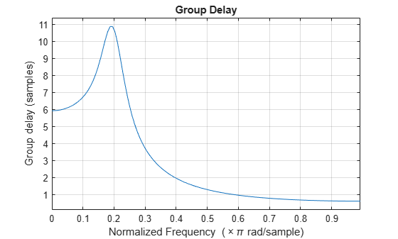
Design a Butterworth filter of order 6 with normalized 3 dB frequency rad/sample. Use grpdelay to display the group delay.
[z,p,k] = butter(6,0.2);
sos = zp2sos(z,p,k);

grpdelay(sos,128)
Plot both the group delay and the phase delay of the system on the same figure.
gd = grpdelay(sos,512);

[h,w] = freqz(sos,512);
pd = -unwrap(angle(h))./w;

plot(w/pi,gd,w/pi,pd)
grid
xlabel("Normalized Frequency (\times\pi rad/sample)")
ylabel("Group and phase delays")
legend(["Group delay" "Phase delay"])

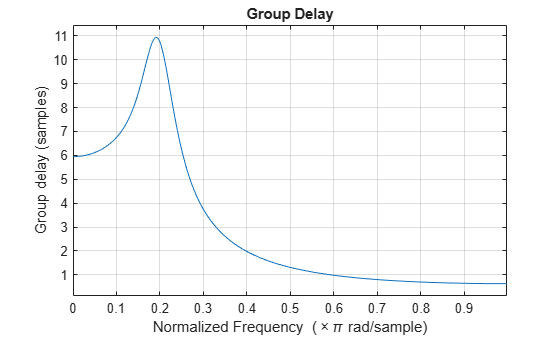
Use designfilt to design a sixth-order Butterworth Filter with normalized 3 dB frequency rad/sample. Display its group delay response.
d = designfilt("lowpassiir",FilterOrder=6, ...
    HalfPowerFrequency=0.2,DesignMethod="butter");
grpdelay(d)
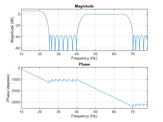
Design an 88th-order FIR filter of arbitrary magnitude response. The filter has two passbands and two stopbands. The lower-frequency passband has twice the gain of the higher-frequency passband. Specify a sample rate of 200 Hz. Visualize the magnitude response and the phase response of the filter from 10 Hz to 78 Hz.
fs = 200;
d = designfilt('arbmagfir', ...
       'FilterOrder',88, ...
       'NumBands',4, ...
       'BandFrequencies1',[0 20], ...
       'BandFrequencies2',[25 40], ...
       'BandFrequencies3',[45 65], ...
       'BandFrequencies4',[70 100], ...
       'BandAmplitudes1',[2 2], ...
       'BandAmplitudes2',[0 0], ...
       'BandAmplitudes3',[1 1], ...
       'BandAmplitudes4',[0 0], ...
       'SampleRate',fs);
freqz(d,10:1/fs:78,fs)
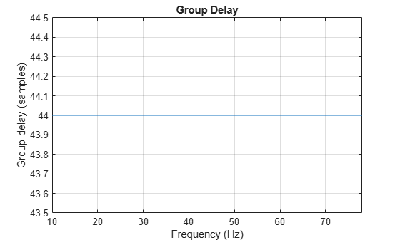
Compute and display the group delay response of the filter over the same frequency range. Verify that it is one-half of the filter order.
filtord(d)
ans =
88
grpdelay(d,10:1/fs:78,fs)
Since R2024b
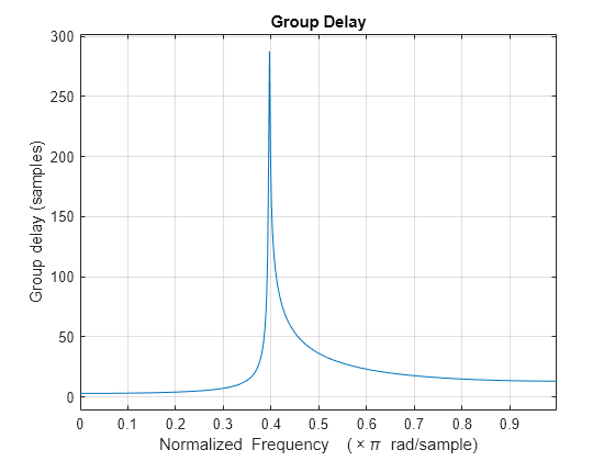
Design a 40th-order lowpass Chebyshev type II digital filter with a stopband edge frequency of 0.4 and stopband attenuation of 50 dB. Plot the group delay response of the filter using its coefficients in the CTF format.
[B,A] = cheby2(40,50,0.4,"ctf");

grpdelay(B,A,"ctf")
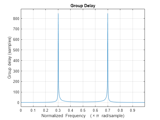
Design a 30th-order bandpass elliptic digital filter with passband edge frequencies of 0.3 and 0.7, passband ripple of 0.1 dB, and stopband attenuation of 50 dB. Plot the group delay response of the filter using its coefficients and gain in the CTF format.
[B,A,g] = ellip(30,0.1,50,[0.3 0.7],"ctf");
grpdelay({B,A,g},"ctf")
Input Arguments
Output Arguments
More About
Tips
You can obtain filters in
CTF format, including the scaling gain. Use the outputs of digital IIR filter design functions,
such as butter, cheby1, cheby2, and ellip. Specify the "ctf" filter-type argument in these
functions and specify to return B, A, and
g to get the scale values. (since R2024b)
References
[1] Lyons, Richard G. Understanding Digital Signal Processing. Upper Saddle River, NJ: Prentice Hall, 2004.
Extended Capabilities
Version History
Introduced before R2006aSee Also
Apps
Functions
ctffilt|cceps|designfilt|digitalFilter|fft|freqz|hilbert|icceps|phasedelay|rceps