freqz
Frequency response of digital filter
Syntax
Description
freqz(___) with
no output arguments plots the frequency response of the filter.
Examples
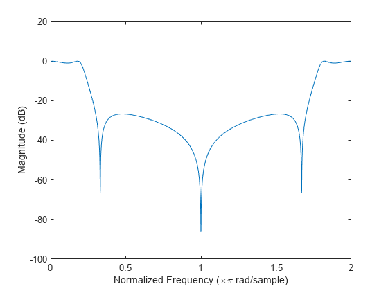
Compute and display the magnitude response of the third-order IIR lowpass filter described by the following transfer function:
Express the numerator and denominator as polynomial convolutions. Find the frequency response at 2001 points spanning the complete unit circle.
b0 = 0.05634;
b1 = [1  1];
b2 = [1 -1.0166 1];
a1 = [1 -0.683];
a2 = [1 -1.4461 0.7957];

b = b0*conv(b1,b2);
a = conv(a1,a2);

[h,w] = freqz(b,a,"whole",2001);
Plot the magnitude response expressed in decibels.
plot(w/pi,20*log10(abs(h)))
ax = gca;
ax.YLim = [-100 20];
ax.XTick = 0:.5:2;
xlabel("Normalized Frequency (\times\pi rad/sample)")
ylabel("Magnitude (dB)")
Since R2024b
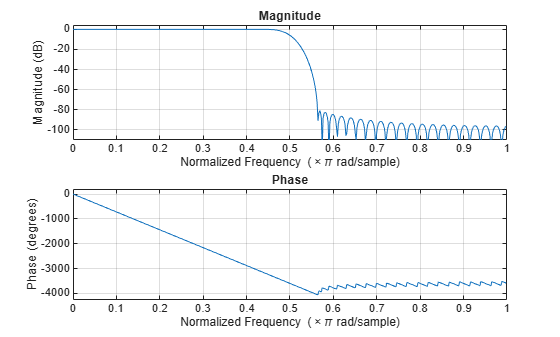
Design a 40th-order lowpass Chebyshev type II digital filter with a stopband edge frequency of 0.4 and stopband attenuation of 50 dB. Plot the frequency response of the filter using its coefficients in the CTF format.
[B,A] = cheby2(40,50,0.4,"ctf");

freqz(B,A,"ctf")
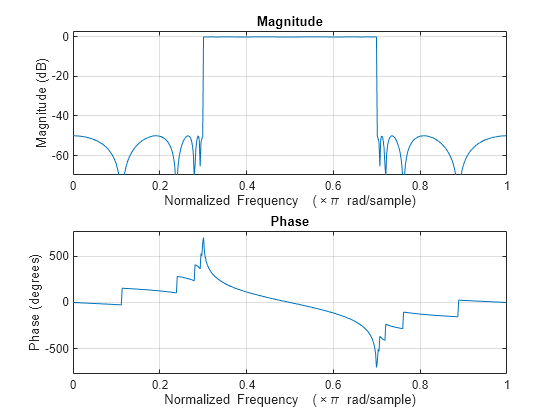
Design a 30th-order bandpass elliptic digital filter with passband edge frequencies of 0.3 and 0.7, passband ripple of 0.1 dB, and stopband attenuation of 50 dB. Plot the frequency response of the filter using its coefficients and gain in the CTF format.
[B,A,g] = ellip(30,0.1,50,[0.3 0.7],"ctf");
freqz({B,A,g},"ctf")
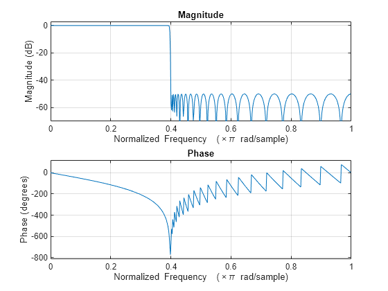
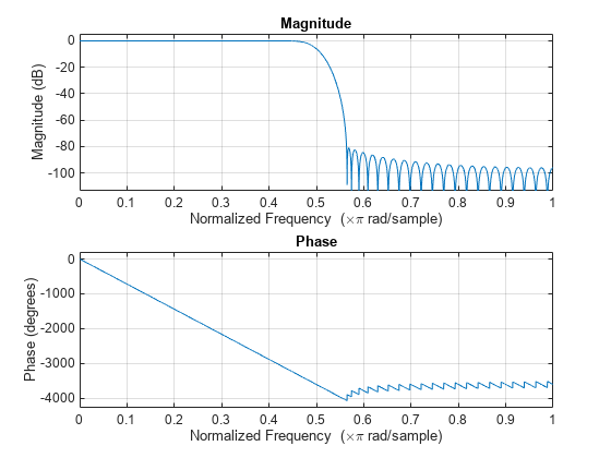
Design an FIR lowpass filter of order 80 using a Kaiser window with . Specify a normalized cutoff frequency of rad/sample. Display the magnitude and phase responses of the filter.
b = fir1(80,0.5,kaiser(81,8));
freqz(b,1)
Design the same filter using designfilt. Display its magnitude and phase responses.
d = designfilt("lowpassfir",FilterOrder=80, ...
    CutoffFrequency=0.5,Window={"kaiser",8});
freqz(d)
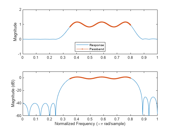
Design an FIR bandpass filter with passband between and rad/sample and 3 dB of ripple. The first stopband goes from to rad/sample and has an attenuation of 40 dB. The second stopband goes from rad/sample to the Nyquist frequency and has an attenuation of 30 dB. Compute the frequency response. Plot its magnitude in both linear units and decibels. Highlight the passband.
sf1 = 0.1;
pf1 = 0.35;
pf2 = 0.8;
sf2 = 0.9;
pb = linspace(pf1,pf2,1e3)*pi;

bp = designfilt("bandpassfir", ...
    StopbandAttenuation1=40,StopbandFrequency1=sf1, ...
    PassbandFrequency1=pf1,PassbandRipple=3, ...
    PassbandFrequency2=pf2,StopbandFrequency2=sf2, ...
    StopbandAttenuation2=30);

[h,w] = freqz(bp,1024);
hpb = freqz(bp,pb);

subplot(2,1,1)
plot(w/pi,abs(h),pb/pi,abs(hpb),'.-')
axis([0 1 -1 2])
legend("Response","Passband",Location="south")
ylabel("Magnitude")

subplot(2,1,2)
plot(w/pi,db(h),pb/pi,db(hpb),".-")
axis([0 1 -60 10])
xlabel("Normalized Frequency (\times\pi rad/sample)")
ylabel("Magnitude (dB)")
Compute and display the magnitude response of the third-order IIR lowpass filter described by the following transfer function:
Express the transfer function in terms of second-order sections. Find the frequency response at 2001 points spanning the complete unit circle.
b0 = 0.05634;
b1 = [1  1];
b2 = [1 -1.0166 1];
a1 = [1 -0.683];
a2 = [1 -1.4461 0.7957];

sos1 = [b0*[b1 0] [a1 0]];
sos2 = [b2 a2];

[h,w] = freqz([sos1;sos2],'whole',2001);
Plot the magnitude response expressed in decibels.
plot(w/pi,20*log10(abs(h)))
ax = gca;
ax.YLim = [-100 20];
ax.XTick = 0:.5:2;
xlabel('Normalized Frequency (\times\pi rad/sample)')
ylabel('Magnitude (dB)')

Input Arguments
Output Arguments
More About
Tips
You can obtain filters in CTF format, including the scaling gain. Use the outputs of digital IIR filter design functions, such as
butter,cheby1,cheby2, andellip. Specify the"ctf"filter-type argument in these functions and specify to returnB,A, andgto get the scale values. (since R2024b)If you have an irreducible multirate filter, use the
freqzmr(DSP System Toolbox) function to analyze the filter in the frequency domain. For more information on irreducible multirate filters, see Overview of Multirate Filters (DSP System Toolbox). (since R2024a)The
freqzmr(DSP System Toolbox) function requires DSP System Toolbox™. (since R2024a)
Algorithms
The frequency response of a digital filter can be interpreted as the transfer function evaluated at z = ejω [1].
freqz determines the transfer function from
the (real or complex) numerator and denominator polynomials you specify
and returns the complex frequency response, H(ejω),
of a digital filter. The frequency response is evaluated at sample
points determined by the syntax that you use.
freqz generally uses an FFT algorithm to compute the frequency response
whenever you do not supply a vector of frequencies as an input argument. It computes the
frequency response as the ratio of the transformed numerator and denominator
coefficients, padded with zeros to the desired length.
When you do supply a vector of frequencies as input, freqz evaluates the
polynomials at each frequency point and divides the numerator response by the
denominator response. To evaluate the polynomials, the function uses Horner's
method.
References
[1] Oppenheim, Alan V., and Ronald W. Schafer, with John R. Buck. Discrete-Time Signal Processing. 2nd Ed. Upper Saddle River, NJ: Prentice Hall, 1999.
[2] Lyons, Richard G. Understanding Digital Signal Processing. Upper Saddle River, NJ: Prentice Hall, 2004.