Verification of Neural Networks

R2026b

This topic shows how to use AI Verification Library for Deep Learning Toolbox™ to verify deep neural networks for safety-critical applications.

Engineers increasingly incorporate neural networks into safety-critical applications, including self-driving cars, diagnostic tools evaluating medical scans, and therapeutic AI language models. As a result, regulators and industries are working together to develop new industry-specific safety standards including standards for AI models.

Neural networks must reliably give correct answers as well as recognize their own uncertainty. Engineers must also be able to measure and confirm the reliability of their networks. In MATLAB^®, you can verify properties of your neural network using the AI Verification Library for Deep Learning Toolbox support package. The support package includes functions to test and improve the robustness of your neural network and to perform out-of-distribution detection.

The full verification workflow can include a variety of tools. The following two links provide examples of the end-to-end workflow.

• For a video showing how to verify a medical imaging classification model, see Understanding and Verifying Your AI Models.

• For an example showing how to approach the certification of an airborne deep learning system that must comply with aviation industry standards such as DO-178C and ARP-4754, see Verify an Airborne Deep Learning System.

Formal Verification

Formal verification uses mathematically rigorous methods to prove or disprove that a system satisfies a specified property for all possible inputs within a defined domain. Unlike testing, which evaluates a finite set of examples, formal verification provides guarantees about the behavior of the system over an entire input region.

Formal verification of a neural network uses mathematical techniques such as abstract interpretation and bound propagation. These techniques can prove properties such as robustness and stability, or provide output bounds without relying on stochastic sampling and test data alone.

Stability and robustness are both measures of how susceptible a neural network is to input perturbations. A network is stable if the network output does not change drastically due to small changes in the network input. A network is robust if it is both stable and correct.

The operational design domain (ODD) is the space of all valid inputs to a network. A neural network can be locally stable or robust within a subsection of the ODD, or it can be globally stable or robust across the entire ODD. Depending on your use case, you may have a requirement on the maximum change in network output given a maximum change in network input, or vice versa. Formal verification methods allow you to prove or disprove whether a neural network satisfies these requirements.

You can formally verify four properties:

• Local stability — A neural network is locally stable within a region centered around a point when inputs close to that point produce outputs that are close to each other.

  $$|x-x_0{|}_p\le ϵ\Rightarrow |f(x)-f(x_0){|}_p\le \delta$$

• Global stability — A neural network is globally stable across the entire ODD if it is locally stable at every point in the ODD.

  $$\forall x_i,x_j\in D\text{ |}{x}_i-x_j{|}_p\le ϵ\Rightarrow |f(x_i)-f(x_j){|}_p\le \delta$$

• Local robustness — A neural network is locally robust within a region centered around a point when inputs close to that point produce outputs that remain close to the ground-truth value at that point.

  $$|x-x_0{|}_p\le ϵ\Rightarrow |f(x)-y_{true}(x_0){|}_p\le \delta$$

• Global robustness — A neural network is globally robust across the entire ODD if it is locally robust at every point in the ODD.

  $$\forall x_i,x_j\in D\text{ |}{x}_i-x_j{|}_p\le ϵ\Rightarrow |f(x_i)-y_{true}(x_j){|}_p\le \delta$$

In these equations, D is the operational design domain, f is the neural network function, y_true is the ground truth, and $$|...{|}_p$$ denotes the choice of norm.

Neural Network Robustness

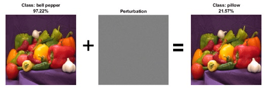
Robustness measures how much the predictions of a neural network change with perturbations to the input data.

Neural networks can be susceptible to a phenomenon called adversarial examples [1]. You can generate adversarial examples by applying small perturbations to examples from the training data such that the model output is incorrect. These perturbations can be small enough to be imperceptible to a human. The Generate Untargeted and Targeted Adversarial Examples for Image Classification example demonstrates how to calculate perturbations that result either in a random wrong answer, or a particular wrong answer for an image classification algorithm.

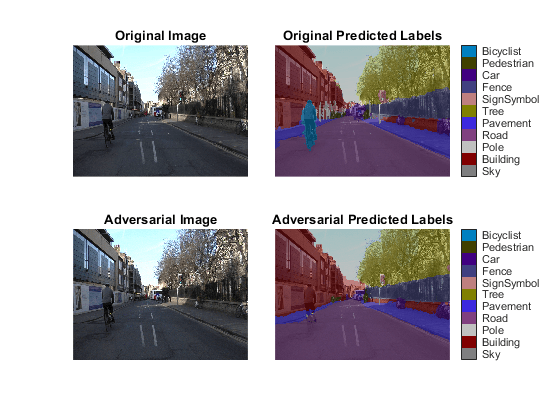
This behavior can have safety ramifications, both intentionally (through a targeted attack) and unintentionally (through random chance). The Generate Adversarial Examples for Semantic Segmentation example demonstrates how to generate adversarial examples for a network that uses semantic segmentation to identify different elements in images of road traffic. In the example, an imperceptible perturbation causes the neural network to misclassify a cyclist on an image of a road.

Measure Robustness

The Verify Robustness of Deep Learning Neural Network example shows how to verify the adversarial robustness of a deep learning neural network.

The AI Verification Library for Deep Learning Toolbox support package includes two functions to measure the robustness of a neural network. For classification models, use verifyNetworkRobustness. For regression models, use estimateNetworkOutputBounds.

Both functions calculate bounds on the range of outputs of a neural network given a range of inputs. They are both based on the DeepPoly algorithm [2]. DeepPoly uses a mix of interval arithmetic and propagation of constraint polyhedra to rigorously compute the output bounds of a network. Statistical techniques, based on sampling a random subset of inputs within a given input perturbation size, can strictly disprove robustness only for a given bound. DeepPoly, by contrast, can strictly prove robustness as well. The computations DeepPoly performs are different for different layers of a neural network. For some layers, the algorithm finds exact bounds. For other layers, the algorithm finds only upper limits to the bounds. If those upper limits are within the desired maximum output, then the network is robust. However, if those upper limits are larger than the desired maximum output, then robustness is unproven.

The verifyNetworkRobustness function checks whether the network classifies all outputs for a given input range as the same class. The function has three possible outputs.

• "verified" — The network is robust to adversarial inputs between the specified bounds.

• "violated" — The network is not robust to adversarial inputs between the specified bounds.

• "unproven" — The function cannot prove whether the network is robust to adversarial inputs between the specified bounds.

The function verifies the network using the final layer. For most applications, use the final fully connected layer for verification. If your network has a softmax layer as the final layer, then the function ignores it and uses the layer before it for verification instead.

The estimateNetworkOutputBounds function computes the range of output values that a network returns when the input is between the specified lower and upper bounds.

Measure Robustness of Pretrained Image Classification Network

Use the verifyNetworkRobustness function to test the robustness of a pretrained image classification network.

load("digitsRobustClassificationMLPNetwork.mat");
[XTest,TTest] = digitTest4DArrayData;
X = XTest(:,:,:,1:10);
label = TTest(1:10);
X = dlarray(X,"SSCB");
perturbation = 0.01;
XLower = X - perturbation;
XUpper = X + perturbation;
result = verifyNetworkRobustness(netRobust,XLower,XUpper,label);
summary(result,Statistics="counts")

result: 10×1 categorical

     verified      10 
     violated       0 
     unproven       0 

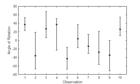
Use the estimateNetworkOutputBounds function to estimate the output bounds of a pretrained regression network.

load("digitsRegressionMLPNetwork.mat");
[XTest,~,TTest] = digitTest4DArrayData;
X = dlarray(XTest(:,:,:,1:10),"SSCB"); 
T = TTest(1:10);
perturbation = 0.01;
XLower = X - perturbation; 
XUpper = X + perturbation;
[YLower,YUpper] = estimateNetworkOutputBounds(net,XLower,XUpper);

Plot the resulting estimates.

YLower = extractdata(YLower);
YUpper = extractdata(YUpper);
figure
errorbar(1:10,T,T-YLower',YUpper'-T,"k*")
axis padded
xlabel("Observation")
ylabel("Angle of Rotation")

Improve Robustness

You can use several methods to improve the robustness of your neural network.

The Train Image Classification Network Robust to Adversarial Examples example shows how to train a neural network that is robust to adversarial examples using fast gradient sign method (FGSM) adversarial training. In adversarial training, you apply adversarial perturbations to the training data during the training process. The network learns how to classify the perturbed images correctly and therefore is more robust to adversarial examples.

The Train Robust Deep Learning Network with Jacobian Regularization example shows how to train a neural network that is robust to adversarial examples using a Jacobian regularization scheme in a custom training loop. In this example, you augment the training data by adding random noise. Then you add a term to the loss function that penalizes the network for large changes in the prediction with respect to small changes in the input.

Out-of-Distribution Detection

Input data that is qualitatively different from training data still results in an output, as long as the format is correct. For example, consider a classification network that classifies images as "cat" or "cucumber." If you ask the network to classify an image of a dog, the network is likely to classify it as "cat," since a dog is in most ways much more similar to a cat than a cucumber.

To determine whether the output of your neural network is meaningful for a given input, you can classify the input data into in-distribution and out-of-distribution data.

In-distribution (ID) data is any data that you use to construct and train your model. Additionally, any data that is sufficiently similar to the training data is also said to be ID.

Out-of-distribution (OOD) data is data that is sufficiently different from the training data, for example, data collected in a different way, at a different time, under different conditions, or for a different task than the data on which the model was originally trained. Models can receive OOD data when you deploy them in an environment other than the one in which you train them. For example, suppose you train a model on high-resolution X-ray images but then deploy the model on images taken with a lower quality camera.

Out-of-distribution detection algorithms work by calculating a confidence score and comparing it to a threshold. You can manually choose this threshold. You can also use AI Verification Library for Deep Learning Toolbox to calculate the threshold based on one of several statistical techniques. To do so, use the networkDistributionDiscriminator function. The function returns a discriminator object that contains information about the network, the algorithm used to calculate the confidence scores, and the threshold used to separate data into ID and OOD.

The Out-of-Distribution Detection for Deep Neural Networks example uses a pretrained classification network and softmax scores to determine if data is ID or OOD. The example also compares different ways of determining the distribution threshold.

The Out-of-Distribution Data Discriminator for YOLO v4 Object Detector example trains an object detector and creates a distribution discriminator object using the histogram-based outlier scores (HBOS) method for the confidence scores and a true positive goal for the threshold determination.

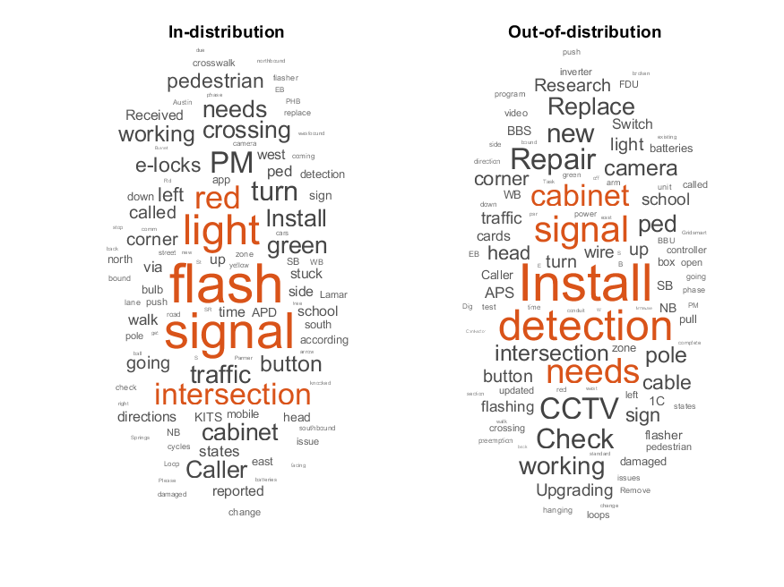
The Out-of-Distribution Detection for LSTM Document Classifier example trains a document classifier and compares different distribution discrimination algorithms to determine whether text data is ID or OOD.

Calculate Confidence Scores

You can use several types of metrics for computing distribution confidence scores. Two such metrics are softmax-based and density-based methods.

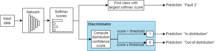
Softmax-based methods use the softmax preactivations, that is, the inputs to the softmax layer, to compute the scores. You can use this class of methods only for classification networks. AI Verification Library for Deep Learning Toolbox provides the baseline method, ODIN method, and energy method.

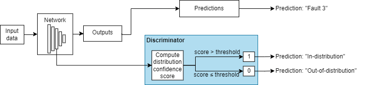
Density-based methods use the probability density functions or layer activations to compute the scores. You can use this class of methods on different types of network architectures. AI Verification Library for Deep Learning Toolbox provides the HBOS and KDE method.

For more information on softmax-based methods and density-based methods, see Distribution Confidence Scores.

The following diagrams show examples of softmax-based and density-based discriminators.

Example of Softmax-Based Discriminator	Example of Density-Based Discriminator

Compare Different Distribution Detection Algorithms

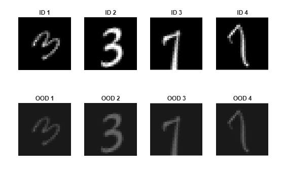
AI Verification Library for Deep Learning Toolbox provides four distribution confidence score algorithms: the baseline method, energy method, ODIN method, HBOS, and KDE method. Compare the behavior of these methods by using them on the same data. First, load the ID data, a set of images of handwritten digits. Modify the ID training data to create an OOD set.

XID = digitTrain4DArrayData;
XOOD = XID.*0.3 + 0.1;

Compare the ID and OOD data.

figure
tiledlayout(2,4,Padding="compact")
for i = 1:4
nexttile(i)
    imshow(XID(:,:,:,i))
    title("ID "+i)
    nexttile(4+i)
    imshow(XOOD(:,:,:,i))
    title("OOD "+i)
end

Next, load a network pretrained on the XID data set and create the discriminator object using the networkDistributionDiscriminator function. To determine whether your data is ID or OOD, pass the discriminator object to the isInNetworkDistribution function. To calculate the distribution scores of your data, pass the discriminator object to the distributionScores function. The function uses the algorithm specified by the "Method" property of the discriminator.

Baseline Distribution Discriminator

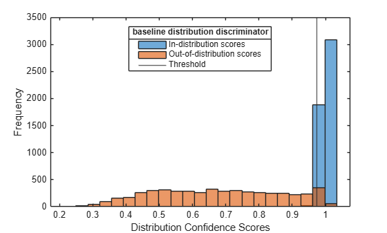
The BaselineDistributionDiscriminator object uses the baseline method to compute distribution confidence scores. The baseline method uses the softmax scores to compute the confidence scores. Predictions with high softmax scores have high baseline confidence scores.

Load a classification network pretrained on the ID data set. Create the discriminator.

load("digitsClassificationMLPNetwork.mat");
discriminatorBaseline = networkDistributionDiscriminator(net,XID,XOOD,"baseline")

discriminatorBaseline = 
  BaselineDistributionDiscriminator with properties:

       Method: "baseline"
      Network: [1×1 dlnetwork]
    Threshold: 0.9743

To assess the performance of the discriminator on the OOD data, calculate the TPR and FPR.

tfOODBaseline = isInNetworkDistribution(discriminatorBaseline,XOOD);
tfIDBaseline = isInNetworkDistribution(discriminatorBaseline,XID);
TPRBaseline = nnz(tfIDBaseline)/numel(tfIDBaseline)

TPRBaseline = 
0.9856

FPRBaseline = nnz(tfOODBaseline)/numel(tfOODBaseline)

FPRBaseline = 
0.0598

To compare the distribution scores of the ID and OOD data, use the plotDistributionScores function, defined at the end of this example.

scoresIDBaseline = distributionScores(discriminatorBaseline,XID);
scoresOODBaseline = distributionScores(discriminatorBaseline,XOOD);
figure
plotDistributionScores(discriminatorBaseline,scoresIDBaseline,scoresOODBaseline)

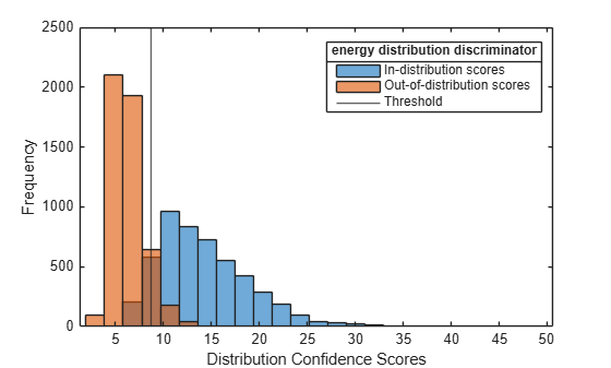
Energy Distribution Discriminator

The EnergyDistributionDiscriminator object is a distribution discriminator that uses the energy method to compute distribution confidence scores. It is a softmax-based method. To tune the algorithm, use the Temperature name-value argument.

Load a classification network pretrained on the ID data set. Create the discriminator. Set Temperature to 0.1.

load("digitsClassificationMLPNetwork.mat");
discriminatorEnergy = networkDistributionDiscriminator(net,XID,XOOD,"energy", ...
Temperature=0.1)

discriminatorEnergy = 
  EnergyDistributionDiscriminator with properties:

         Method: "energy"
        Network: [1×1 dlnetwork]
    Temperature: 0.1000
      Threshold: 8.7246

To assess the performance of the discriminator on the OOD data, calculate the TPR and FPR.

tfOODEnergy = isInNetworkDistribution(discriminatorEnergy,XOOD);
tfIDEnergy = isInNetworkDistribution(discriminatorEnergy,XID);
TPREnergy = nnz(tfIDEnergy)/numel(tfIDEnergy)

TPREnergy = 
0.9106

FPREnergy = nnz(tfOODEnergy)/numel(tfOODEnergy)

FPREnergy = 
0.0934

To compare the distribution scores of the ID and OOD data, use the plotDistributionScores function, defined at the end of this example.

scoresIDEnergy = distributionScores(discriminatorEnergy,XID);
scoresOODEnergy = distributionScores(discriminatorEnergy,XOOD);
figure
plotDistributionScores(discriminatorEnergy,scoresIDEnergy,scoresOODEnergy)

ODIN Distribution Discriminator

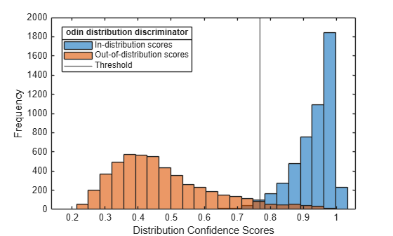
The ODINDistributionDiscriminator object enables you to compute distribution confidence scores by using the out-of-distribution detector for neural networks (ODIN) method. It is a softmax-based method. Similar to the energy distribution discriminator, the method is based on a rescaling of the softmax scores parameterized by the Temperature name-value argument. When the Temperature parameter is 1, the ODIN distribution discriminator is equal to the baseline distribution discriminator.

Load a classification network pretrained on the ID data set. Create the discriminator. Set Temperature to 2.

load("digitsClassificationMLPNetwork.mat");
discriminatorODIN = networkDistributionDiscriminator(net,XID,XOOD,"odin", ...
Temperature=2)

discriminatorODIN = 
  ODINDistributionDiscriminator with properties:

         Method: "odin"
        Network: [1×1 dlnetwork]
    Temperature: 2
      Threshold: 0.7687

To assess the performance of the discriminator on the OOD data, calculate the TPR and FPR.

tfOODODIN = isInNetworkDistribution(discriminatorODIN,XOOD);
tfIDODIN = isInNetworkDistribution(discriminatorODIN,XID);
TPRODIN = nnz(tfIDODIN)/numel(tfIDODIN)

TPRODIN = 
0.9766

FPRODIN = nnz(tfOODODIN)/numel(tfOODODIN)

FPRODIN = 
0.0558

To compare the distribution scores of the ID and OOD data, use the plotDistributionScores function, defined at the end of this example.

scoresIDODIN = distributionScores(discriminatorODIN,XID);
scoresOODODIN = distributionScores(discriminatorODIN,XOOD);
figure
plotDistributionScores(discriminatorODIN,scoresIDODIN,scoresOODODIN)

HBOS Distribution Discriminator

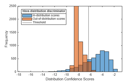
The HBOSDistributionDiscriminator object uses the histogram based outlier scores (HBOS) method to compute distribution confidence scores and is a density-based method. Density-based methods compute distribution scores by describing the underlying features learned by the network as probabilistic models. Observations falling into areas of low density correspond to OOD observations.

The HBOS algorithm assumes that the features are statistically independent. The principal component features are pairwise linearly independent but they can have nonlinear dependencies. To investigate feature dependencies, you can use functions such as corr (Statistics and Machine Learning Toolbox) (Statistics and Machine Learning Toolbox). For an example showing how to investigate feature dependence, see Out-of-Distribution Data Discriminator for YOLO v4 Object Detector. If the features are not statistically independent, then the algorithm can return poor results. Using multiple layers to compute the distribution scores can increase the number of statistically dependent features.

You can use the HBOS distribution discriminator on different types of network architectures, including regression networks.

Load a regression network pretrained on the ID data set. Create the discriminator. Use the penultimate layer to compute the HBOS distribution scores. Set the VarianceCutoff value to 0.05.

load("digitsRegressionMLPNetwork.mat");
discriminatorHBOS = networkDistributionDiscriminator(net,XID,XOOD,"hbos", ...
VarianceCutoff=0.05, ...
LayerNames="relu_2")

discriminatorHBOS = 
  HBOSDistributionDiscriminator with properties:

            Method: "hbos"
           Network: [1×1 dlnetwork]
        LayerNames: "relu_2"
    VarianceCutoff: 0.0500
         Threshold: -6.2918

To assess the performance of the discriminator on the OOD data, calculate the TPR and FPR.

tfOODHBOS = isInNetworkDistribution(discriminatorHBOS,XOOD);
tfIDHBOS = isInNetworkDistribution(discriminatorHBOS,XID);
TPRHBOS = nnz(tfIDHBOS)/numel(tfIDHBOS)

TPRHBOS = 
0.7334

FPRHBOS = nnz(tfOODHBOS)/numel(tfOODHBOS)

FPRHBOS = 
0.0508

To compare the distribution scores of the ID and OOD data, use the plotDistributionScores function, defined at the end of this example.

scoresIDHBOS = distributionScores(discriminatorHBOS,XID);
scoresOODHBOS = distributionScores(discriminatorHBOS,XOOD);
figure
plotDistributionScores(discriminatorHBOS,scoresIDHBOS,scoresOODHBOS)

KDE Distribution Discriminator

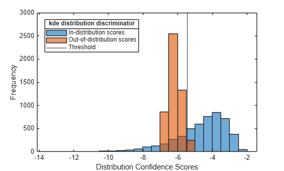
The KDEDistributionDiscriminator object uses kernel density estimation (KDE) to compute distribution confidence scores and is another density-based method. The KDE method has the same assumptions and underlying behavior of the HBOS method. The key difference is that instead of estimating the underlying density with histograms, it uses kernel density estimates. The KDE discriminator can produce a smoother approximation of the distribution scores than HBOS, at the cost of being more computationally expensive to create. For deployment, it is recommended to use KDE to reduce changes in OOD classification decisions.

Using a KDE discriminator requires Statistics and Machine Learning Toolbox™.

Load a regression network pretrained on the ID data set. Create the discriminator. Use the penultimate layer to compute the KDE distribution scores. Set the VarianceCutoff value to 0.05.

load("digitsRegressionMLPNetwork.mat");
discriminatorKDE = networkDistributionDiscriminator(net,XID,XOOD,"kde", ...
VarianceCutoff=0.05, ...
LayerNames="relu_2")

discriminatorKDE = 
  KDEDistributionDiscriminator with properties:

            Method: "kde"
           Network: [1×1 dlnetwork]
        LayerNames: "relu_2"
    VarianceCutoff: 0.0500
         Threshold: -5.4559

To assess the performance of the discriminator on the OOD data, calculate the TPR and FPR.

tfOODKDE = isInNetworkDistribution(discriminatorKDE,XOOD);
tfIDKDE = isInNetworkDistribution(discriminatorKDE,XID);
TPRKDE = nnz(tfIDKDE)/numel(tfIDKDE)

TPRKDE = 
0.7570

FPRKDE = nnz(tfOODKDE)/numel(tfOODKDE)

FPRKDE = 
0.0374

To compare the distribution scores of the ID and OOD data, use the plotDistributionScores function, defined at the end of this example.

scoresIDKDE = distributionScores(discriminatorKDE,XID);
scoresOODKDE = distributionScores(discriminatorKDE,XOOD);
figure
plotDistributionScores(discriminatorKDE,scoresIDKDE,scoresOODKDE)

Supporting Function

This function plots a histogram of ID distribution scores and OOD distribution scores.

function plotDistributionScores(discriminator,scoresID,scoresOOD)
    hID = histogram(scoresID);
    hold on
    hOOD = histogram(scoresOOD);
    xl = xlim;
    hID.BinWidth = (xl(2)-xl(1))/25;
    hOOD.BinWidth = (xl(2)-xl(1))/25;
    xline(discriminator.Threshold)
    l = legend(["In-distribution scores","Out-of-distribution scores","Threshold"],Location="best");
    title(l,discriminator.Method+" distribution discriminator")
    xlabel("Distribution Confidence Scores")
    ylabel("Frequency")
    hold off
end

Calculate Out-of-Distribution Threshold

After you calculate the distribution scores of your data, compare them to a threshold to decide whether your data is in-distribution or out-of-distribution.

Manual Threshold

One option is to choose a threshold manually. For the baseline scores, you can use the isInNetworkDistribution function and pass the network, the data, and the threshold as input arguments. In this case, the function normalizes the threshold to lie between 0 and 1.

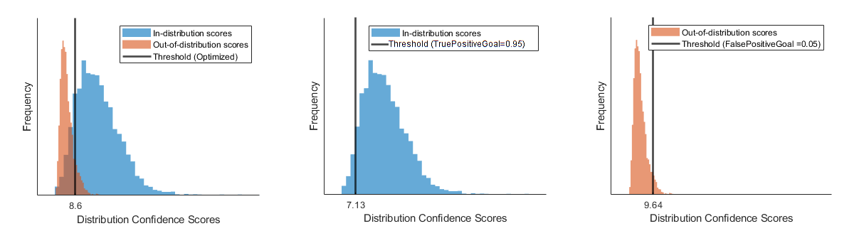
Optimal Threshold

You can also measure the quality of a threshold by the TPR and FPR. A good discriminator has a TPR close to 1 and an FPR close to 0.

The networkDistributionDiscriminator function calculates an optimal threshold. The optimization metric depends on the inputs.

If you provide only ID data to the networkDistributionDiscriminator function, or if you set the TruePositiveGoal name-value argument, then the function returns the threshold that correctly classifies at least this proportion of the ID data as ID, while keeping the false positive rate as low as possible. The default true positive goal is 0.95.

discriminatorOnlyID = networkDistributionDiscriminator(net,XID,[],"baseline");
discriminatorTPG = networkDistributionDiscriminator(net,XID,XOOD,"baseline",TruePositiveGoal=0.95);
discriminatorOnlyID.Threshold
discriminatorTPG.Threshold

If you provide only OOD data to the networkDistributionDiscriminator function, or if you set the FalsePositiveGoal name-value argument in the input, then the function returns the threshold that incorrectly classifies at most this proportion of the OOD data as ID, while keeping the true positive rate as high as possible. The default false positive goal is 0.05.

discriminatorOnlyOOD = networkDistributionDiscriminator(net,[],XOOD,"baseline");
discriminatorFPG = networkDistributionDiscriminator(net,XID,XOOD,"baseline",FalsePositiveGoal=0.05);
discriminatorOnlyOOD.Threshold
discriminatorFPG.Threshold

If you provide both ID and OOD data and do not specify a true or false positive goal, then networkDistributionDiscriminator maximizes the TPR while minimizing the FPR by maximizing the following expression: $$\frac{1}{2}(TPR+(1-FPR))$$.

discriminatorIDAndOOD = networkDistributionDiscriminator(net,XID,XOOD,"baseline");
discriminatorIDAndOOD.Threshold

This figure illustrates the different thresholds that the discriminator chooses if you optimize over both the true positive rate and false positive rate, just the true positive rate, or just the false positive rate.

Other Techniques

You can use other techniques to verify the behavior of your neural network in MATLAB beyond the robustness and OOD detection methods included in AI Verification Library for Deep Learning Toolbox.

Interpretability and Visualization

One way of verifying the behavior of your network is to understand its decision-making process by using interpretability techniques.

The AI Verification Library for Deep Learning Toolbox support package includes the drise function. Use this function to calculate the saliency map to explain the predictions of an object detection network by using the detector randomized input sampling for explanation (D-RISE) algorithm.

For more information about interpreting machine learning models, see Interpret Machine Learning Models (Statistics and Machine Learning Toolbox).

For an overview of deep learning visualization methods, see Deep Learning Visualization Methods

Anomaly Detection

OOD detection typically takes advantage of the features of your trained neural network to determine whether input data is ID or OOD. You can also use statistical anomaly detection techniques directly on your input data to determine whether your data is significantly dissimilar to your training data. For more information on anomaly detection in MATLAB, see Anomaly Detection.

You can also use the HBOS or KDE distribution detectors to determine whether your data is ID or OOD based only on the data. To do this, set the LayerNames name-value argument in the networkDistributionDiscriminator function to the input layer of your network.

Uncertainty Estimation

Uncertainty estimation is important in safety critical applications, where the AI system must be able to generalize over unseen data, and the uncertainty associated with the AI model predictions must be accounted for in way that does not compromise on safety. For more information about uncertainty estimation for regression models, see Uncertainty Estimation for Regression (Statistics and Machine Learning Toolbox) and Create Prediction Intervals Using Split Conformal Prediction (Statistics and Machine Learning Toolbox).

References

[1] Goodfellow, Ian J., Jonathon Shlens, and Christian Szegedy. “Explaining and Harnessing Adversarial Examples.” Preprint, submitted March 20, 2015. https://doi.org/10.48550/arXiv.1412.6572.

[2] Singh, Gagandeep, Timon Gehr, Markus Püschel, and Martin Vechev. “An Abstract Domain for Certifying Neural Networks”. Proceedings of the ACM on Programming Languages 3, no. POPL (January 2, 2019): 1–30. https://doi.org/10.1145/3290354.