Generate Untargeted and Targeted Adversarial Examples for Image Classification

This example shows how to use the fast gradient sign method (FGSM) and the basic iterative method (BIM) to generate adversarial examples for a pretrained neural network.

Neural networks can be susceptible to a phenomenon known as adversarial examples [1], where very small changes to an input can cause the input to be misclassified. These changes are often imperceptible to humans.

In this example, you create two types of adversarial examples:

• Untargeted — Modify an image so that it is misclassified as any incorrect class.

• Targeted — Modify an image so that it is misclassified as a specific class.

Load Network and Image

Load a network that has been trained on the ImageNet [2] data set.

[net, classNames] = imagePretrainedNetwork;
inputSize = net.Layers(1).InputSize(1:2);

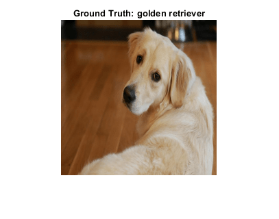
Load a test image and resize it to the expected network input size. This is an image of a golden retriever.

img = imread("sherlock.jpg");
groundTruth = categorical("golden retriever",classNames);

img = imresize(img,inputSize);
X = dlarray(single(img),"SSCB");

Find the predicted class of the image.

score = predict(net,X);
YTest = scores2label(score,classNames)

YTest = categorical
     golden retriever 

View the test image.

figure
imshow(img)

Untargeted Fast Gradient Sign Method

Create an adversarial example using the untargeted FGSM [3]. This method calculates the gradient $${\nabla }_{X}L\left(X,T\right)$$ of the loss function $$L$$, with respect to the image $$X$$ you want to find an adversarial example for. This gradient describes the direction to "push" the image in to increase the chance it is misclassified. You can then add or subtract a small error from each pixel to increase the likelihood the image is misclassified.

The adversarial example is calculated as follows:

$X_{\text{adv}}=X+\alpha .\text{sign}\left({\nabla }_{X}L\left(X,T\right)\right)$.

Parameter $\alpha$ is the step size and controls the size of the push. A larger $\alpha$ value increases the chance of generating a misclassified image, but makes the change in the image more visible. This method is untargeted, as the aim is to get the image misclassified, regardless of which class.

Generate lower and upper bounds between which to search for the adversarial image. As the image has values in the range [0,255], ensure that the values do not go below 0 or above 255.

epsilon = 1;

XLower = max(X-epsilon,0);
XUpper = min(X+epsilon,255);

Use the adversarialOptions object to set the step size to 2. To generate valid images, use an integer step size.

optionsFGSM = adversarialOptions("fgsm",Stepsize=2);

Use the findAdversarialExamples function to find an adversarial example. If the epsilon value is large enough, then the function returns an adversarial example. Otherwise, the function returns []. Because the algorithm includes randomness, the function may return different results each time you run it. If the function is unable to find an adversarial example, try changing the options or running the function again.

[example,mislabel] = findAdversarialExamples(net,XLower,XUpper,groundTruth,Algorithm=optionsFGSM);

Display the original image and the adversarial image. The network correctly classifies the unaltered image as a golden retriever. However, because of perturbation, the network misclassifies the adversarial image. Once added to the image, the perturbation is imperceptible, demonstrating how adversarial examples can exploit robustness issues within a network.

figure
tiledlayout(1,2);

nexttile(1);
imshow(img);
title({"Original Image","Predicted Label: " + string(classNames(YTest))});

nexttile(2)
imshow(uint8(extractdata(example)));
title({"Adversarial Example", "Predicted Label: " + string(classNames(mislabel))});

Targeted Adversarial Examples

A simple improvement to the FGSM is to perform multiple iterations. This approach is known as the basic iterative method (BIM) [4] or projected gradient descent [5]. This method can yield adversarial examples with less distortion than the FGSM.

When you use the untargeted FGSM, the predicted label of the adversarial example can be very similar to the label of the original image. For example, a dog might be misclassified as a different kind of dog. However, you can easily modify these methods to misclassify an image as a specific class.

Generate a targeted adversarial example using the BIM with the number of iterations set to 30 and a step size of 1.

optionsBIM = adversarialOptions("bim",NumIterations=30,StepSize=1);

Set the target class to "great white shark" and increase the epsilon value to 5.

targetClass = categorical("great white shark",classNames);

epsilon = 5;
XLower = max(X-epsilon,0);
XUpper = min(X+epsilon,255);

Using the BIM, generate a new adversarial example. Note that you may have to adjust these settings for other networks.

[example,mislabel] = findAdversarialExamples(net,XLower,XUpper,groundTruth,Algorithm=optionsBIM,AdversarialLabel=targetClass);

Display the targeted adversarial image. Because of imperceptible perturbation, the network classifies the adversarial image as a great white shark.

figure
tiledlayout(1,2);

nexttile(1);
imshow(img);
title({"Original Image","Predicted Label: " + string(classNames(YTest))});

nexttile(2)
imshow(uint8(extractdata(example)));
title({"Adversarial Example", "Predicted Label: " + string(classNames(mislabel))});

To make the network more robust against adversarial examples, you can use adversarial training. For an example showing how to train a network robust to adversarial examples, see Train Image Classification Network Robust to Adversarial Examples.

References

[1] Goodfellow, Ian J., Jonathon Shlens, and Christian Szegedy. “Explaining and Harnessing Adversarial Examples.” Preprint, submitted March 20, 2015. https://arxiv.org/abs/1412.6572.

[2] ImageNet. http://www.image-net.org.

[3] Szegedy, Christian, Wojciech Zaremba, Ilya Sutskever, Joan Bruna, Dumitru Erhan, Ian Goodfellow, and Rob Fergus. “Intriguing Properties of Neural Networks.” Preprint, submitted February 19, 2014. https://arxiv.org/abs/1312.6199.

[4] Kurakin, Alexey, Ian Goodfellow, and Samy Bengio. “Adversarial Examples in the Physical World.” Preprint, submitted February 10, 2017. https://arxiv.org/abs/1607.02533.

[5] Madry, Aleksander, Aleksandar Makelov, Ludwig Schmidt, Dimitris Tsipras, and Adrian Vladu. “Towards Deep Learning Models Resistant to Adversarial Attacks.” Preprint, submitted September 4, 2019. https://arxiv.org/abs/1706.06083.