distributionScores

Distribution confidence scores

Since R2023a

Syntax

scores = distributionScores(discriminator,X)

scores = distributionScores(discriminator,X1,...,XN)

scores = distributionScores(___,VerbosityLevel=level)

Description

scores = distributionScores(discriminator,X) returns the distribution confidence score for each observation in X using the method you specify in the Method property of discriminator. You can use the scores to separate data into in-distribution (ID) and out-of-distribution (OOD) data sets. For example, you can classify any observation with distribution confidence score less than or equal to the Threshold property of discriminator as OOD. For more information about how the software computes the distribution confidence scores, see Distribution Confidence Scores.

scores = distributionScores(discriminator,X1,...,XN) returns the distribution scores for networks with multiple inputs using the specified in-memory data.

scores = distributionScores(___,VerbosityLevel=level) also specifies the verbosity level.

Examples

Find Distribution Scores

Load a pretrained classification network.

load('digitsClassificationMLPNet.mat');

Load ID data. Convert the data to a dlarray object.

XID = digitTrain4DArrayData;
XID = dlarray(XID,"SSCB");

Modify the ID training data to create an OOD set.

XOOD = XID.*0.3 + 0.1;

Create a discriminator using the networkDistributionDiscriminator function.

method = "baseline";
discriminator = networkDistributionDiscriminator(net,XID,XOOD,method)

discriminator = 
  BaselineDistributionDiscriminator with properties:

       Method: "baseline"
      Network: [1x1 dlnetwork]
    Threshold: 0.9743

The discriminator object contains a threshold for separating the ID and OOD confidence scores.

Use the distributionScores function to find the distribution scores for the ID and OOD data. You can use the distribution confidence scores to separate the data into ID and OOD. The algorithm the software uses to compute the scores is set when you create the discriminator. In this example, the software computes the scores using the baseline method.

scoresID = distributionScores(discriminator,XID);
scoresOOD = distributionScores(discriminator,XOOD);

Plot the distribution confidence scores for the ID and OOD data. Add the threshold separating the ID and OOD confidence scores.

figure
histogram(scoresID,BinWidth=0.02)
hold on
histogram(scoresOOD,BinWidth=0.02)
xline(discriminator.Threshold)
legend(["In-distribution scores","Out-of-distribution scores","Threshold"],Location="northwest")
xlabel("Distribution Confidence Scores")
ylabel("Frequency")
hold off

Assess Performance Using ROC Curve

Load a pretrained classification network.

load("digitsClassificationMLPNet.mat");

Load ID data and convert the data to a dlarray object.

XID = digitTrain4DArrayData;
XID = dlarray(XID,"SSCB");

Modify the ID training data to create an OOD set.

XOOD = XID.*0.3 + 0.1;

Create a discriminator.

method = "baseline";
discriminator = networkDistributionDiscriminator(net,XID,XOOD,method);

Use the distributionScores function to find the distribution scores for the ID and OOD data. You can use the distribution scores to separate the data into ID and OOD.

scoresID = distributionScores(discriminator,XID);
scoresOOD = distributionScores(discriminator,XOOD);

Use rocmetrics to plot a ROC curve to show how well the model performs at separating the data into ID and OOD.

labels = [
    repelem("In-distribution",numel(scoresID)), ...
    repelem("Out-of-distribution",numel(scoresOOD))];
scores = [scoresID',scoresOOD'];

rocObj = rocmetrics(labels,scores,"In-distribution");
figure
plot(rocObj)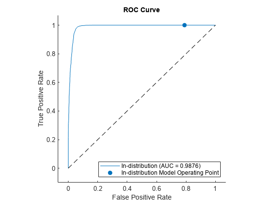

Input Arguments

discriminator — Distribution discriminator

BaselineDistributionDiscriminator object | ODINDistributionDiscriminator object | EnergyDistributionDiscriminator object | HBOSDistributionDiscriminator object

Distribution discriminator, specified as a BaselineDistributionDiscriminator, ODINDistributionDiscriminator, EnergyDistributionDiscriminator, or HBOSDistributionDiscriminator object. To create this object, use the networkDistributionDiscriminator function.

X — Input data

formatted dlarray | minibatchqueue object

Input data, specified as a formatted dlarray or a minibatchqueue object that returns a formatted dlarray. For more information about dlarray formats, see the fmt input argument of dlarray.

Use a minibatchqueue object for a network with multiple inputs where the data does not fit on disk. If you have data that fits in memory that does not require additional processing, then it is usually easiest to specify the input data as in-memory arrays. For more information, see X1,...,XN.

X1,...,XN — In-memory data for multi-input network

formatted dlarray

In-memory data for multi-input network, specified dlarray objects. The input Xi corresponds to the network input discriminator.Network.InputNames(i).

For multi-input networks, if you have data that fits in memory that does not require additional processing, then it is usually easiest to specify the input data as in-memory arrays. If you want to make predictions with data stored on disk, then specify X as a minibatchqueue object.

level — Verbosity level

"off" (default) | "summary" | "detailed"

Verbosity level of the Command Window output, specified as one of these values:

• "off" — Do not display progress information.

• "summary" — Display a summary of the progress information.

• "detailed" — Display detailed information about the progress. This option prints the mini-batch progress. If you do not specify the input data as a minibatchqueue object, then the "detailed" and "summary" options print the same information.

Data Types: char | string

More About

In-Distribution and Out-of-Distribution Data

In-distribution (ID) data refers to any data that you use to construct and train your model. Additionally, any data that is sufficiently similar to the training data is also said to be ID.

Out-of-distribution (OOD) data refers to data that is sufficiently different to the training data. For example, data collected in a different way, at a different time, under different conditions, or for a different task than the data on which the model was originally trained. Models can receive OOD data when you deploy them in an environment other than the one in which you train them. For example, suppose you train a model on clear X-ray images but then deploy the model on images taken with a lower-quality camera.

OOD data detection is important for assigning confidence to the predictions of a network. For more information, see OOD Data Detection.

OOD Data Detection

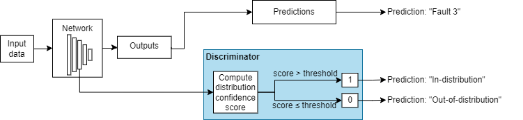
OOD data detection is a technique for assessing whether the inputs to a network are OOD. For methods that you apply after training, you can construct a discriminator which acts as an additional output of the trained network that classifies an observation as ID or OOD.

The discriminator works by finding a distribution confidence score for an input. You can then specify a threshold. If the score is less than or equal to that threshold, then the input is OOD. Two groups of metrics for computing distribution confidence scores are softmax-based and density-based methods. Softmax-based methods use the softmax layer to compute the scores. Density-based methods use the outputs of layers that you specify to compute the scores. For more information about how to compute distribution confidence scores, see Distribution Confidence Scores.

These images show how a discriminator acts as an additional output of a trained neural network.

Example Data Discriminators

Example of Softmax-Based Discriminator	Example of Density-Based Discriminator
For more information, see Softmax-Based Methods.	For more information, see Density-Based Methods.

Distribution Confidence Scores

Distribution confidence scores are metrics for classifying data as ID or OOD. If an input has a score less than or equal to a threshold value, then you can classify that input as OOD. You can use different techniques for finding the distribution confidence scores.

Softmax-Based Methods

ID data usually corresponds to a higher softmax output than OOD data[1]. Therefore, a method of defining distribution confidence scores is as a function of the softmax scores. These methods are called softmax-based methods. These methods only work for classification networks with a single softmax output.

Let a_i(X) be the input to the softmax layer for class i. The output of the softmax layer for class i is given by this equation:

$$P_i(X;T)=\frac{e^{a_i(X)/T}}{{\displaystyle \sum _{j=1}^C{e}^{a_j(X)/T}}},$$

where C is the number of classes and T is a temperature scaling. When the network predicts the class label of X, the temperature T is set to 1.

The baseline, ODIN, and energy methods each define distribution confidence scores as functions of the softmax input.

• The baseline method [1] uses the maximum of the unscaled output values of the softmax scores:

  $$\text{confidence}(X)=\underset{i}{\max }{P}_i(X;1).$$

• The out-of-distribution detector for neural networks (ODIN) method [2] uses the maximum of the scaled output of the softmax scores:

  $$\text{confidence}(X;T)=\underset{i}{\max }{P}_i(X;T)\text{, }T>0.$$

• The energy method [3] uses the scaled denominator of the softmax output:

  $$\begin{array}{l}\text{energy}(X;T)=-T\log \left({\displaystyle \sum _{j=1}^C{e}^{a_j(X)/T}}\right)\text{, }T>0\\ \text{confidence}(X;T)=-\text{energy}(X;T)\text{, }T>0.\end{array}$$

Density-Based Methods

Density-based methods compute the distribution scores by describing the underlying features learned by the network as probabilistic models. Observations falling into areas of low density correspond to OOD observations.

To model the distributions of the features, you can describe the density function for each feature using a histogram. This technique is based on the histogram-based outlier score (HBOS) method [4]. This method uses a data set of ID data, such as training data, to construct histograms representing the density distributions of the ID features. This method has three stages:

1. Find the principal component features for which to compute the distribution confidence scores:

   1. For each specified layer, find the activations using the n data set observations. Flatten the activations across all dimensions except the batch dimension.

   2. Compute the principal components of the flattened activations matrix. Normalize the eigenvalues such that the largest eigenvalue is 1 and corresponds to the principal component that carries the greatest variance through the layer. Denote the matrix of principal components for layer l by Q^(l).

      The principal components are linear combinations of the activations and represent the features that the software uses to compute the distribution scores. To compute the score, the software uses only the principal components whose eigenvalues are greater than the variance cutoff value σ.

      Note

      The HBOS algorithm assumes that the features are statistically independent. The principal component features are pairwise linearly independent but they can have nonlinear dependencies. To investigate feature dependencies, you can use functions such as corr (Statistics and Machine Learning Toolbox). For an example showing how to investigate feature dependence, see Out-of-Distribution Data Discriminator for YOLO v4 Object Detector. If the features are not statistically independent, then the algorithm can return poor results. Using multiple layers to compute the distribution scores can increase the number of statistically dependent features.

2. For each of the principal component features with an eigenvalue greater than σ, construct a histogram. For each histogram:

   1. Dynamically adjusts the width of the bins to create $$\sqrt{n}$$ bins of approximately equal area.

   2. Normalize the bins heights such that the largest height is 1.

3. Find the distribution score for an observation by summing the logarithmic height of the bin containing the observation for each of the feature histograms, over each of the layers.

   Let f^(l)(X) denote the output of layer l for input X. Use the principal components to project the output into a lower dimensional feature space using this equation: $${\widehat{f}}^{(l)}(X)={\left(Q^{(l)}\right)}^T{f}^{(l)}(X)$$.

   Compute the confidence score using this equation:

   $$\begin{array}{l}\text{HBOS}(X;\sigma )=-{\displaystyle \sum _{l=1}^L\left({\displaystyle \sum _{k=1}^{N^{(l)}(\sigma )}\text{log}\left({\text{hist}}_k\left({\widehat{f}}_k^{(l)}(X)\right)\right)}\right)},\\ \text{confidence}(X;\sigma )=-\text{HBOS}(X;\sigma ),\end{array}$$

   where N^(l)(σ) is the number of number of principal component with an eigenvalue less than σ and L is the number of layers. A larger score corresponds to an observation that lies in the areas of higher density. If the observation lies outside of the range of any of the histograms, then the bin height for those histograms is 0 and the confidence score is -Inf.

   Note

   The distribution scores depend on the properties of the data set used to construct the histograms [6].

References

[1] Shalev, Gal, Gabi Shalev, and Joseph Keshet. “A Baseline for Detecting Out-of-Distribution Examples in Image Captioning.” In Proceedings of the 30th ACM International Conference on Multimedia, 4175–84. Lisboa Portugal: ACM, 2022. https://doi.org/10.1145/3503161.3548340.

[2] Shiyu Liang, Yixuan Li, and R. Srikant, “Enhancing The Reliability of Out-of-distribution Image Detection in Neural Networks” arXiv:1706.02690 [cs.LG], August 30, 2020, http://arxiv.org/abs/1706.02690.

[3] Weitang Liu, Xiaoyun Wang, John D. Owens, and Yixuan Li, “Energy-based Out-of-distribution Detection” arXiv:2010.03759 [cs.LG], April 26, 2021, http://arxiv.org/abs/2010.03759.

[4] Markus Goldstein and Andreas Dengel. "Histogram-based outlier score (hbos): A fast unsupervised anomaly detection algorithm." KI-2012: poster and demo track 9 (2012).

[5] Jingkang Yang, Kaiyang Zhou, Yixuan Li, and Ziwei Liu, “Generalized Out-of-Distribution Detection: A Survey” August 3, 2022, http://arxiv.org/abs/2110.11334.

[6] Lee, Kimin, Kibok Lee, Honglak Lee, and Jinwoo Shin. “A Simple Unified Framework for Detecting Out-of-Distribution Samples and Adversarial Attacks.” arXiv, October 27, 2018. http://arxiv.org/abs/1807.03888.

Extended Capabilities

C/C++ Code Generation

Generate C and C++ code using MATLAB® Coder™.

Usage notes and limitations:

• Generated code for distributionScores supports single observations only. To process batches of observations, pass each observation individually.

• To load a discriminator object for code generation, use the coder.loadNetworkDistributionDiscriminator function.

• Requires the MATLAB^® Coder™ Interface for Deep Learning support package. If this support package is not installed, use the Add-On Explorer. To open the Add-On Explorer, go to the MATLAB® Toolstrip and click Add-Ons > Get Add-Ons.

GPU Code Generation

Generate CUDA® code for NVIDIA® GPUs using GPU Coder™.

Usage notes and limitations:

• Generated code for distributionScores supports single observations only. To process batches of observations, pass each observation individually.

• To load a discriminator object for code generation, use the coder.loadNetworkDistributionDiscriminator function.

• Requires the GPU Coder™ Interface for Deep Learning support package. If this support package is not installed, use the Add-On Explorer. To open the Add-On Explorer, go to the MATLAB® Toolstrip and click Add-Ons > Get Add-Ons.

GPU Arrays

Accelerate code by running on a graphics processing unit (GPU) using Parallel Computing Toolbox™.

Usage notes and limitations:

• This function runs on the GPU if its inputs meet either or both of these conditions:

  • Any values of the network learnable parameters are dlarray objects with underlying data of type gpuArray. To see the learnables for a network net, call net.Learnables.Value.

  • Any of the data is a dlarray object with underlying data of type gpuArray.

For more information, see Run MATLAB Functions on a GPU (Parallel Computing Toolbox).

Version History

Introduced in R2023a

R2024a: Use networks with multiple inputs

The distributionScores function now support networks with multiple inputs.

R2023a: Display progress information (June 2023; Version 23.1.1)

Set the VerbosityLevel option to view progress information. The software displays progress information in the Command Window. You can set the VerbosityLevel to "off", "summary", or "detailed".

R2023a: Use minibatchqueue objects (June 2023; Version 23.1.1)

Detect out-of-distribution data using minibatchqueue objects. You can use minibatchequeue objects to create, preprocess, and manage mini-batches of data, and to automatically convert your data to a dlarray object.

R2023a: Code generation support (June 2023; Version 23.1.1)

Generate C or C++ code using MATLAB Coder or generate CUDA^® code for NVIDIA^® GPUs using GPU Coder. For usage notes and limitations, see Extended Capabilities.