Results for
- I open the MQTT Configure block.
- I fill out all the required fields — Broker address, Port, Client ID, Username, and Password.
- When I click Test Connection, it says “Connection established successfully.” So far so good.
- Then I click Apply, close the dialog, set the topic name, and try to run the simulation.
- At this point, I get the following error:Caused by: Invalid value for 'ClientID', 'Username' or 'Password'.
- When I reopen the MQTT config block, I notice that the Password field is empty again — even though I definitely entered it before and the connection test worked earlier.

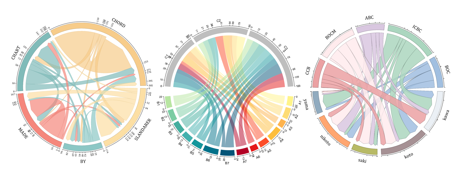
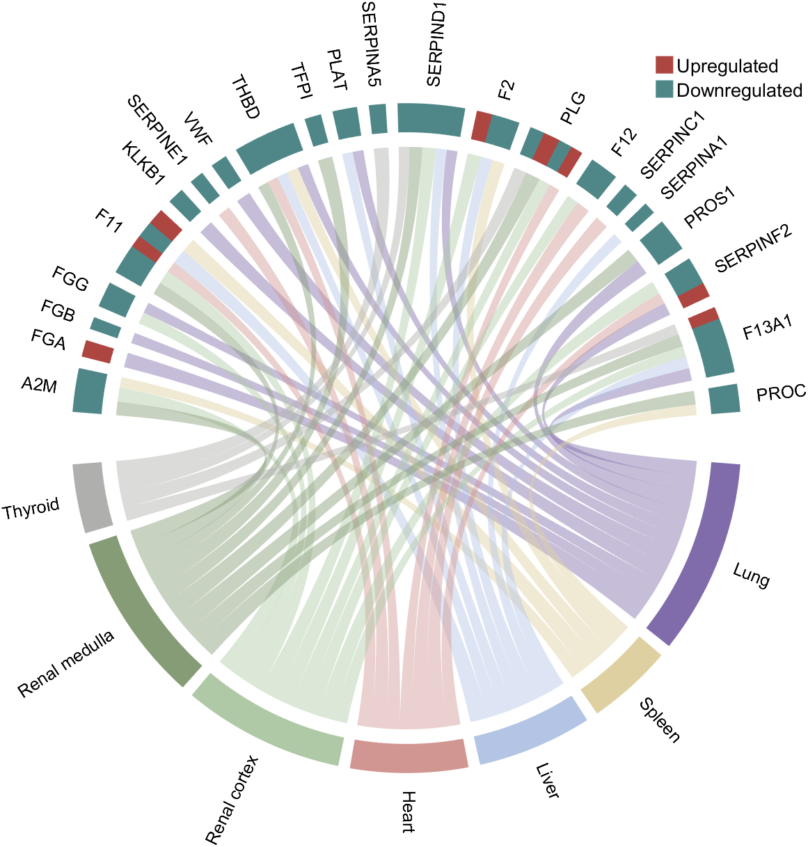
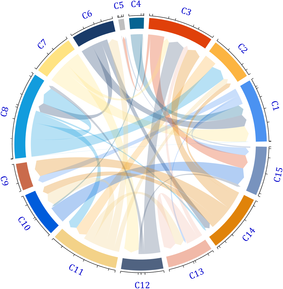
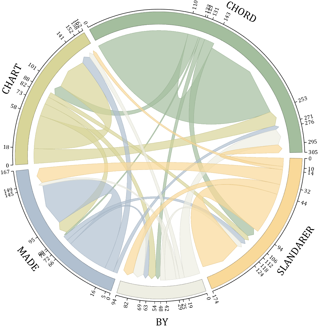
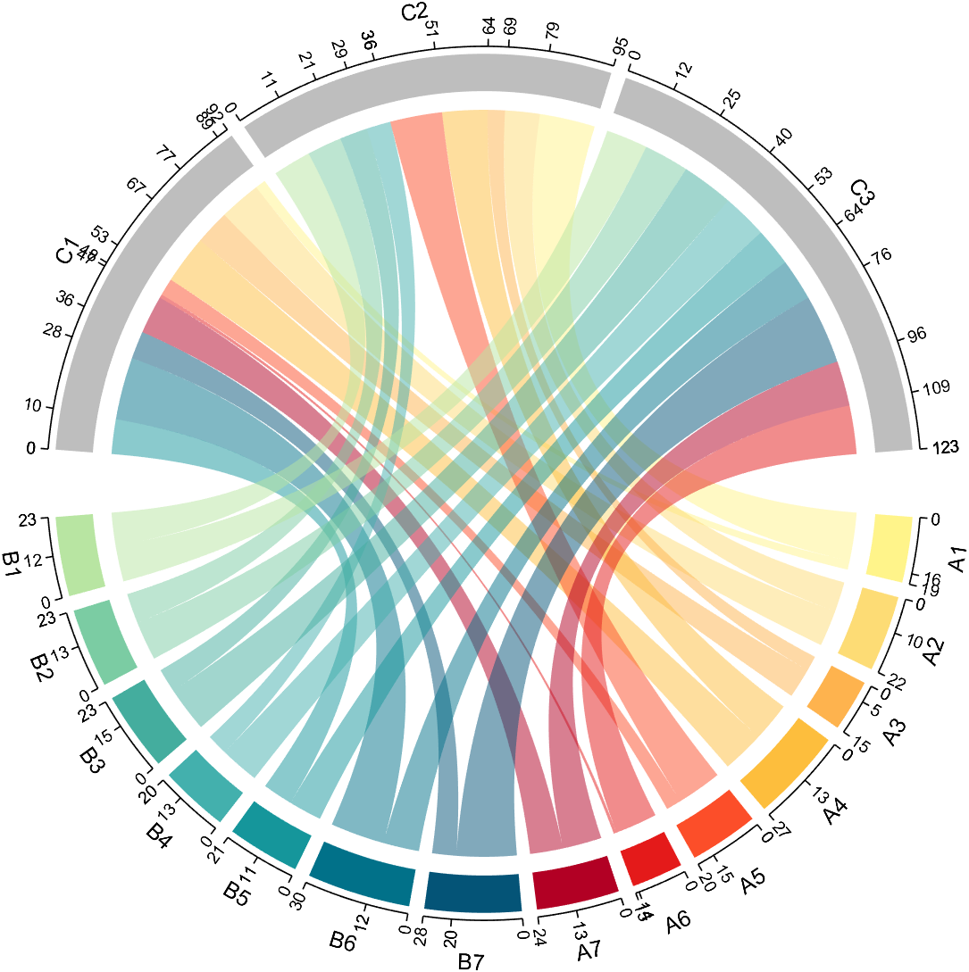
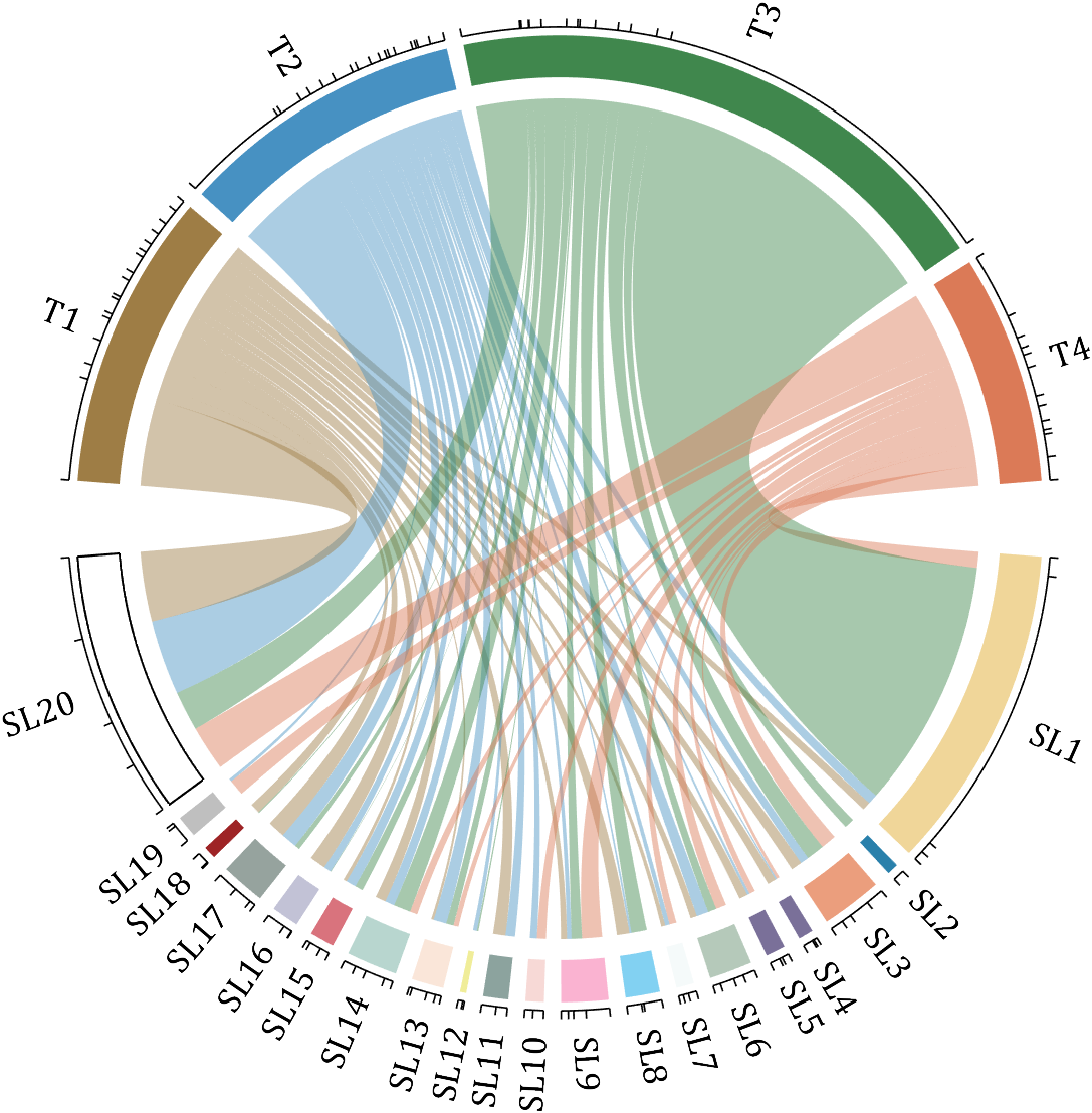
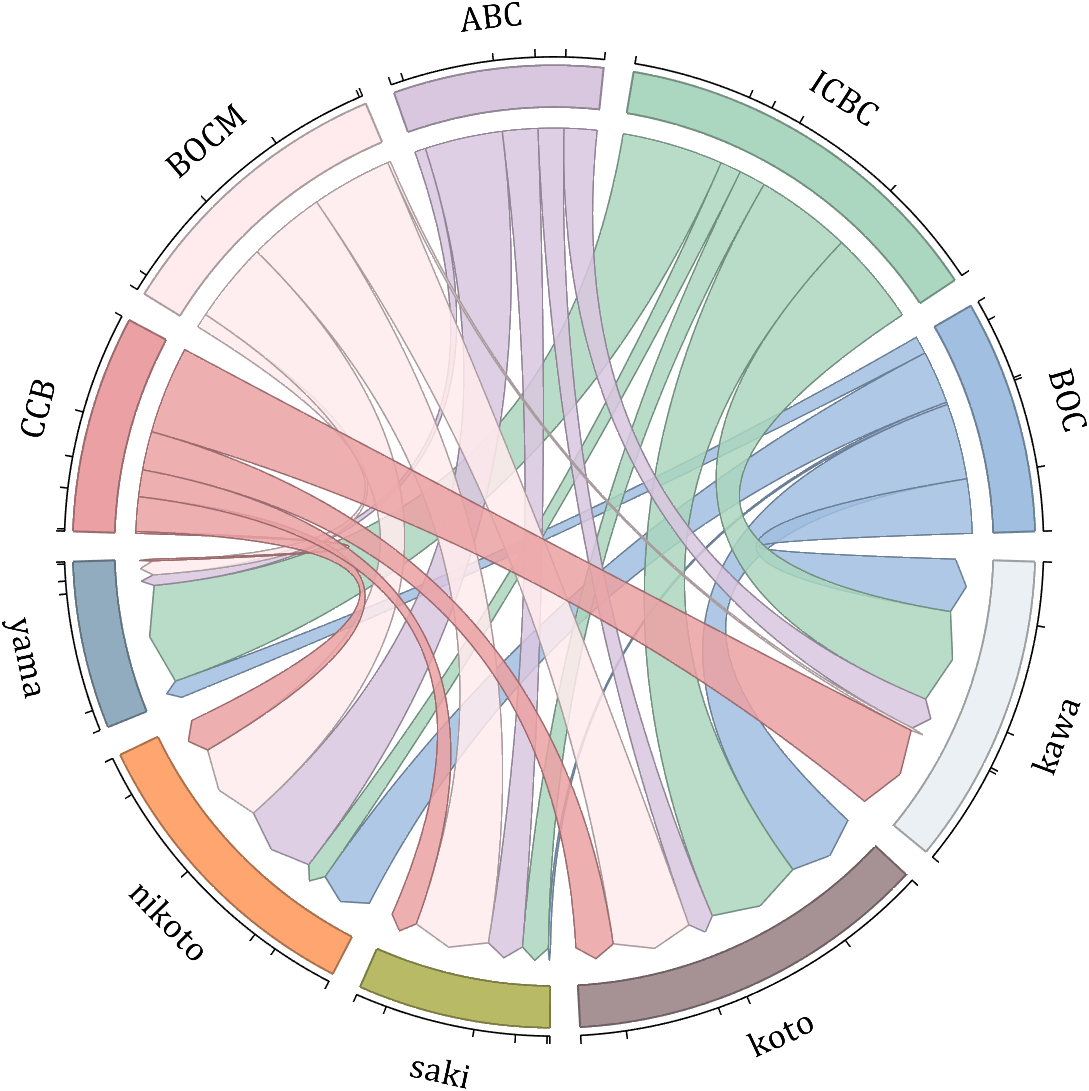
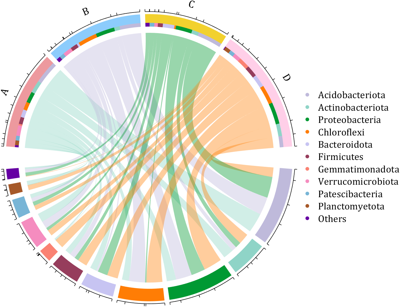
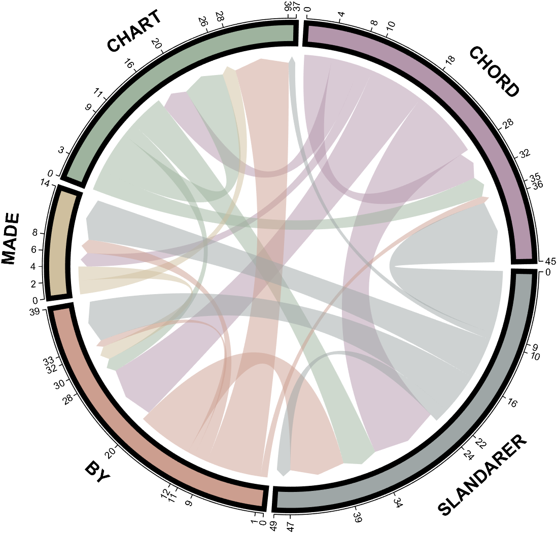
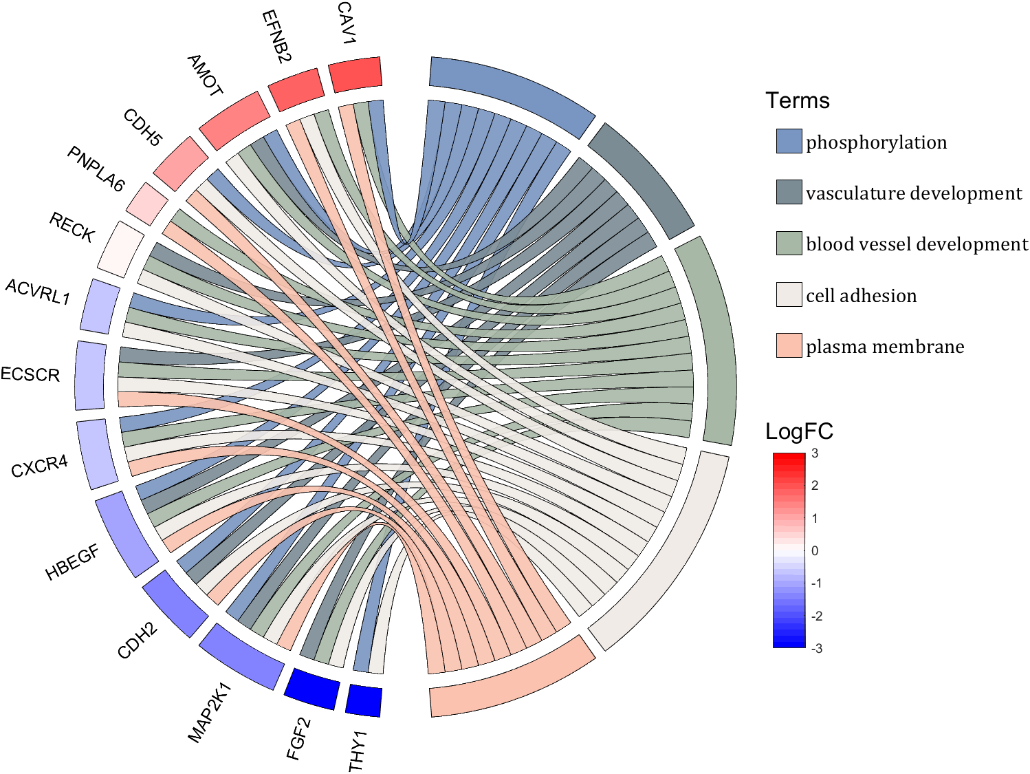
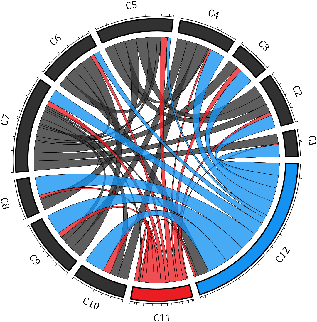
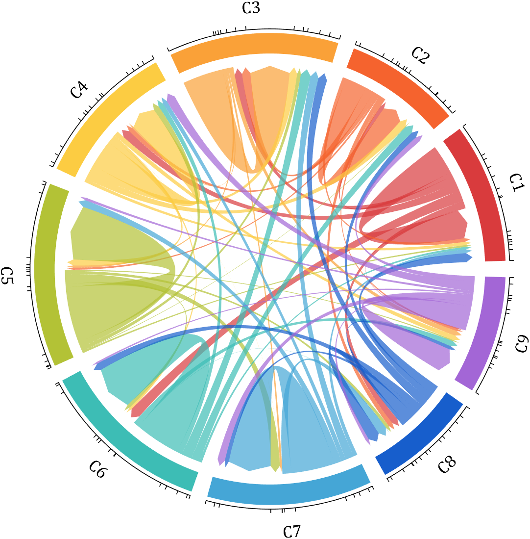
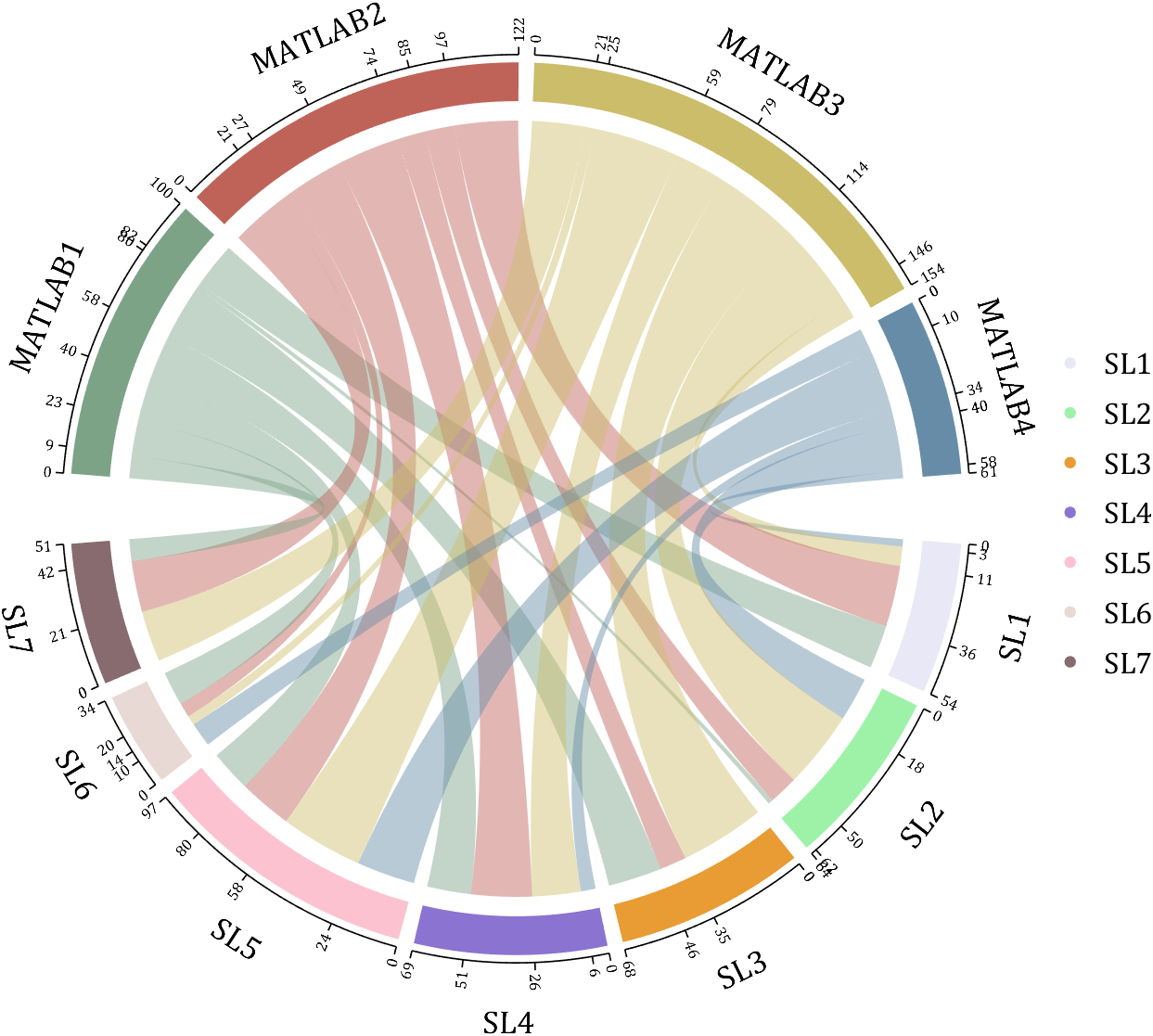
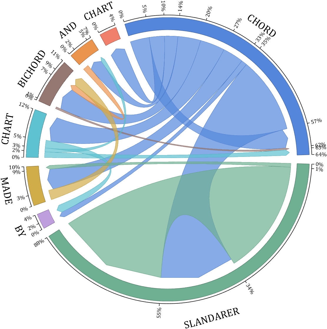
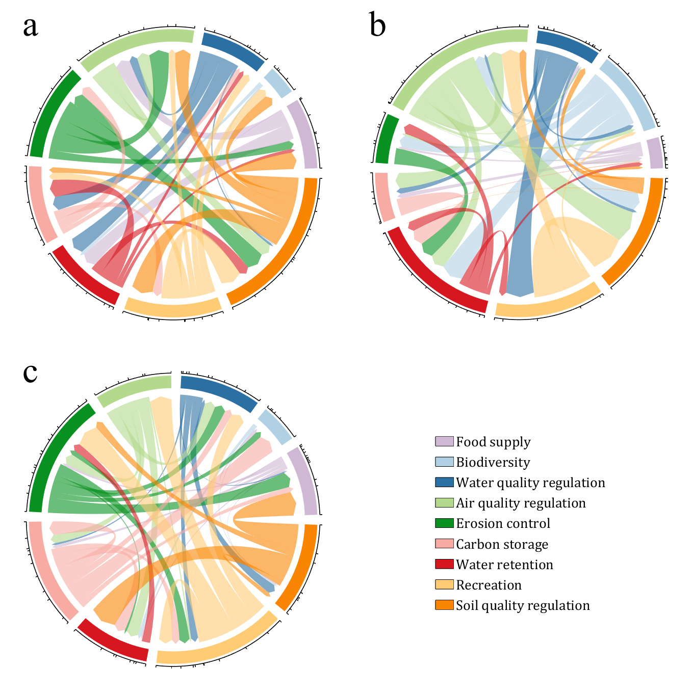
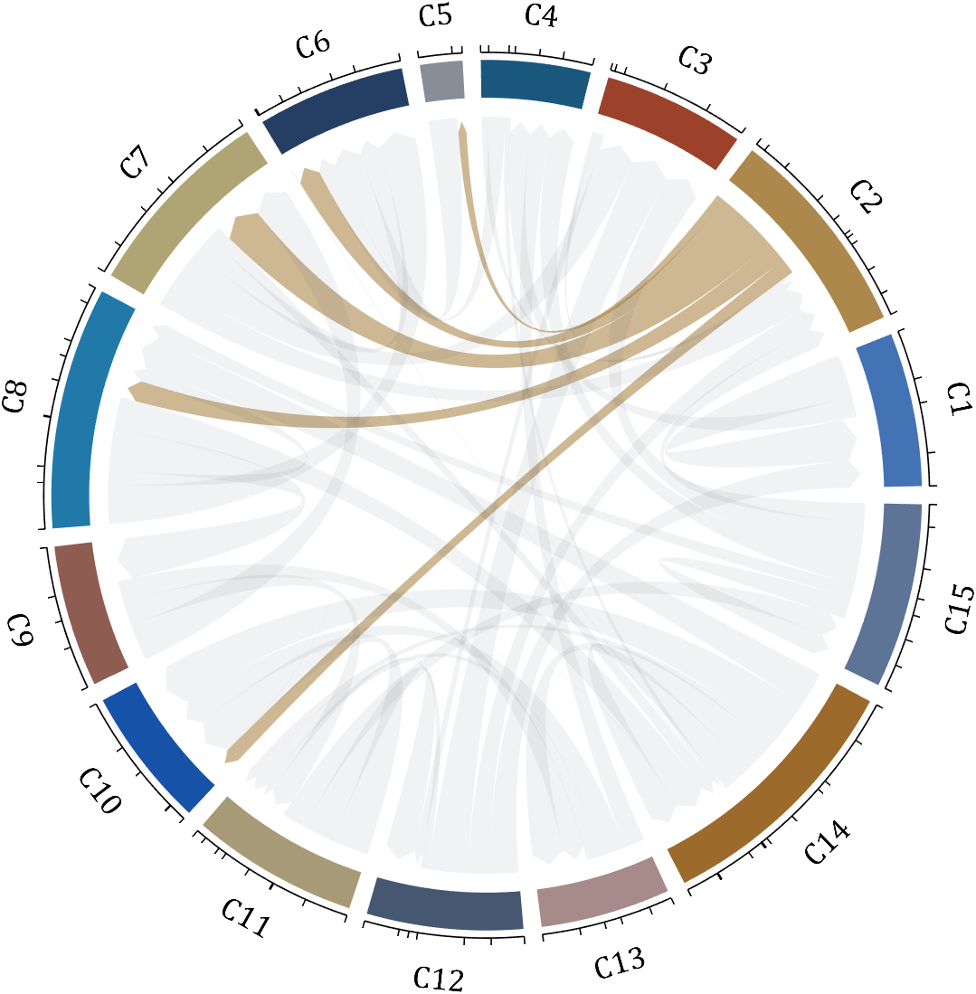
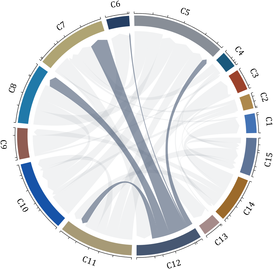
- - Chord chart: [chord chart](https://www.mathworks.com/matlabcentral/fileexchange/116550-chord-chart)
- - Directed graph chord chart: [digraph chord chart]:(https://www.mathworks.com/matlabcentral/fileexchange/121043-digraph-chord-chart)
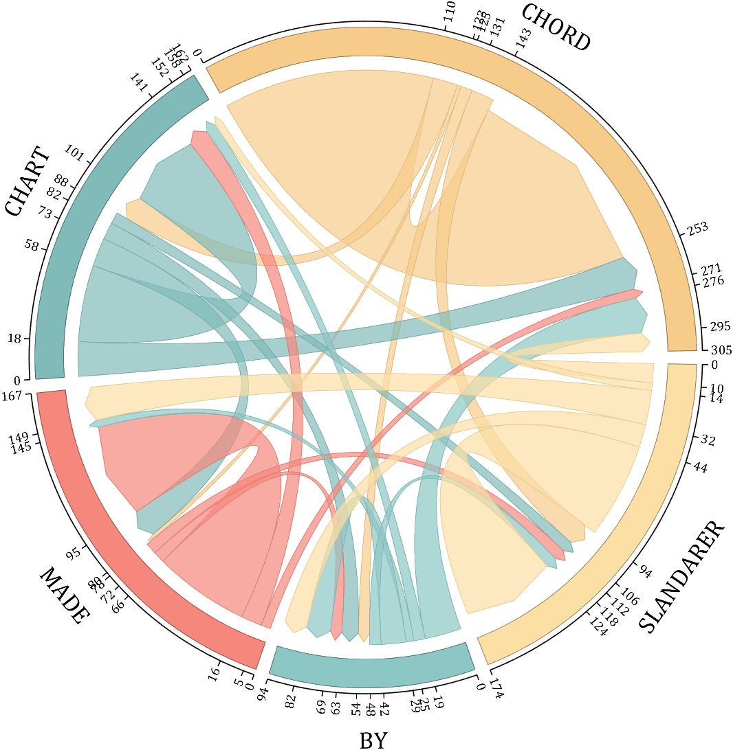
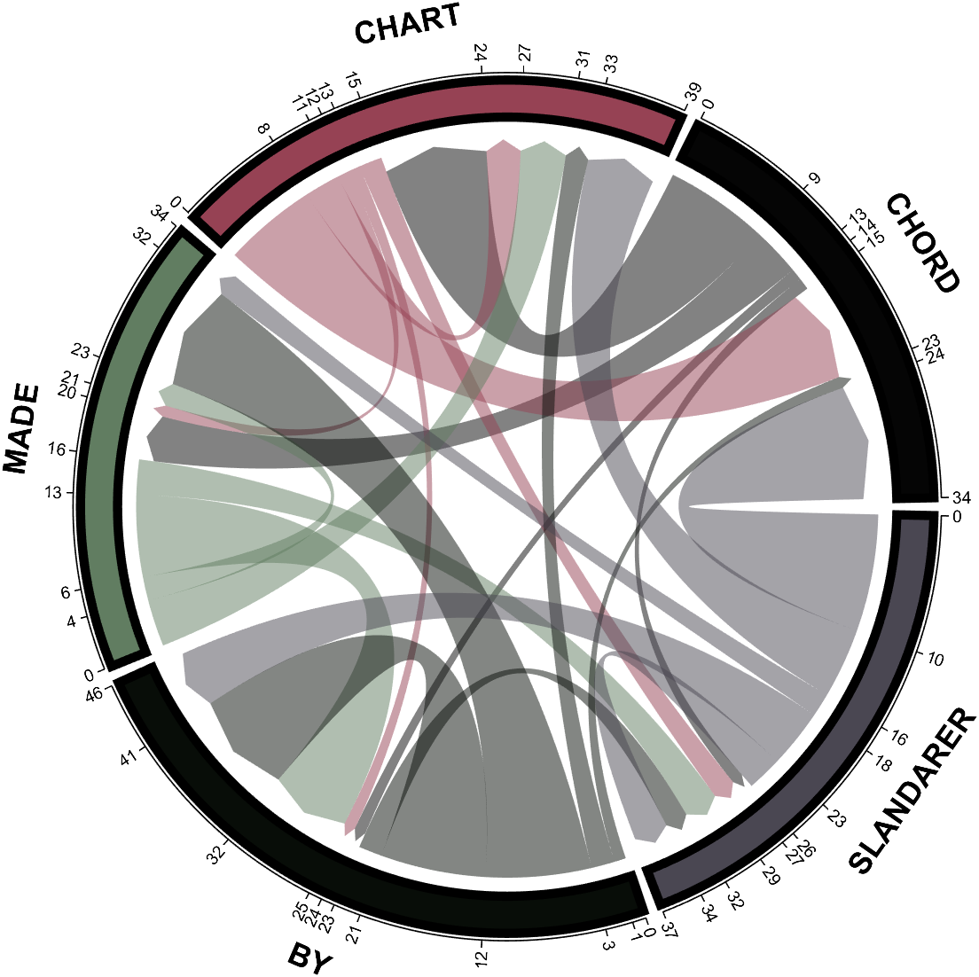
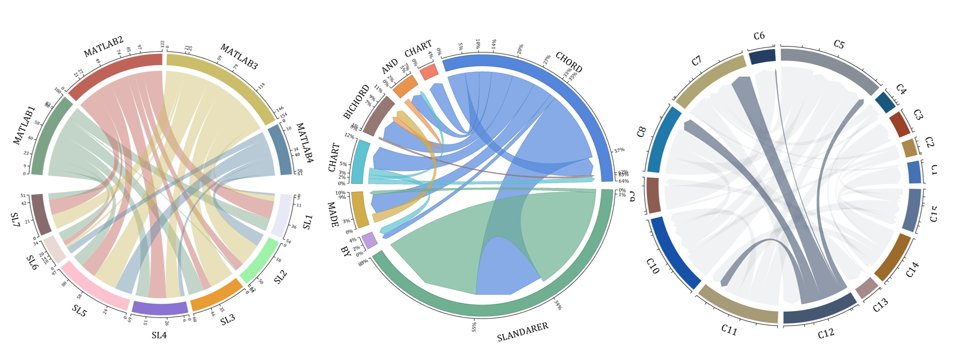
- - Chord chart: [chord chart](https://www.mathworks.com/matlabcentral/fileexchange/116550-chord-chart)
- - Directed graph chord chart: [digraph chord chart]:(https://www.mathworks.com/matlabcentral/fileexchange/121043-digraph-chord-chart)
- Replace the legend with a colorbar to update the location and orientation of the colorbar.
- Define a GridSizeChangedFcn within the loop so that it is called every time a tile is added.
- Create a figure with many tiles (~20) and dynamically set a color to each row of axes.
- Assign xlabels only to the bottom row of tiles and ylabels to only the left column of tiles.
- What happens when all elements of v are equal?
- Can you produce a vector with uniform spacing without using colons or linspace?
- What additional steps would be needed to use isuniform with circular data?
- isuniform - documentation
- Floating point numbers - documentation
- Floating point numbers - Cleve's Corner (blog)
.
MATLAB R2022a provides app developers more control over user navigation through app components using the keyboard's Tab key.
Part 1. The new focus function: programmatically set keyboard focus to a UI component
Part 2. Modify focus order of components
Today we'll review Part 2. See yesterday's Community Highlight for Part 1.
-------------------------------------------------------------------------------------------------
Well-designed apps have an obvious flow through interactive fields and, as we learned yesterday, using the Tab key to move the focus to the next UI component is faster and more efficient than using a mouse. Here we'll learn how to read and set the tab order of UI components in an app.
Understanding tab and stacking order
By default, tab order in MATLAB apps is controlled by the stacking order in the Component Browser. Initially, the stacking order within the component browswer is based on the sequence in which the objects were added to the container object within the app. MATLAB R2020b gave us control to edit the stacking order by selecting a component and using either the Reorder tool from the Canvas toolstrip or by right-clicking the component and selecting Reorder from the context menu [1]. Tab order flows from bottom to top through the Component Browswer hierarchy for objects that are focusable. Sending a component backward within the stack sets its tab order to earlier relative to other components.
Setting tab focus order in R2022a
Three additional tab order features were added in MATLAB R2022a that make it easier to control app navigation with the Tab key.
1. Sort and Filter by Tab Order : Instead of using the Reorder tool which lists components in reverse tab-order and includes components that are not focusable, filter the list by focusable components and sort them by tab-order using the View dropdown menu within the Component Browser (label 1 in image below). From here, you can drag and drop components to set their tab (and stacking) order.
2. Auto Tab Order : To automatically sort focusable components within your app so that the tab order is from left-to-right and then top-to-bottom, in App Designer, from Design View, select the Canvas tab > Tab Order button > Apply Auto Tab Order (label 2 in image below). Alternatively, you can apply auto tab order to components within a container such as a uipanel or uitab by right-clicking on the container within the Component Browser and selecting Apply Auto Tab Order.
3. Visualize Tab Order : You no longer have to read and interpret the handle names in the component browser to understand the current tab order of UI components. Instead, view an animation of tab order within App Designer. From Design View, select the Canvas tab > Tab Order button > Visualize Tab Order (label 3 in image below).
.
Contextual focus control: the power of combining focus() with setting tab order
Yesterday's Community Highlight showed how to programmatically set UI component focus using the focus(c) function. This, combined with control of tab order, allows app developers to implement contextual focus control. For example, when a radio button is selected in the GIF below, the corresponding UI Tab is selected programmatically and the keyboard focus is set to the first component within the UI Tab thus allowing the user to smoothly continue keyboard navigation. This is achieved by a callback function that responds to changes in the Button Group that sets the SelectedTab property of the TabGroup and uses the new focus() function. For details, see the attached focusAndTabOrderDemo.mlapp.
-------------------------------------------------------------------------------------------------
Stay tuned
Follow Community Highlights to get notifications for new content.
Let us know what interests you in the new MATLAB R2022a release in the comment section below.
See also
- MATLAB documentation: Modify Tab Focus Order of Components
- Release notes: Modify tab focus order
- R2021a Highlight: keyboard shortcuts for UI Components
- Download the latest release of MATLAB
Footnotes
[1] R202b release notes: change the stacking order of UI components
This Community Highlight is attached as a live script.
.
MATLAB R2022a provides app developers more control over user navigation through app components using the keyboard's Tab key.
Part 1. The new focus function: programmatically set keyboard focus to a UI component
Part 2. Modify focus order of components
Today we'll review Part 1. Come back tomorrow for Part 2.
-------------------------------------------------------------------------------------------------
Programmatically set UI component focus
Did you know that you can save ~2 seconds every time you use a keyboard shortcut rather than reaching for your mouse [1,2]?
I need you to focus here: starting in MATLAB R2022a, use the new focus function to set keyboard focus to a specific UI component.
By specifying the component handle ( c ) in focus(c),
- The figure containing the component is displayed
- A blue frame appears around the component
- The user can directly interact with the component.
.
Which components are focusable?
Focusable components are those that a user can interact with using the keyboard. So an object set to Enable='off' or Visible='off' cannot be in focus. See the documentation for more details.
What will you do with all of that extra time saved?
-------------------------------------------------------------------------------------------------
Stay tuned
Tomorrow we'll learn how to apply the new focus function with control of tab order to create contextual flow of UI component focus. Follow Community Highlights to get notifications.
Let us know what interests you in the new MATLAB R2022a release in the comment section below.
See also
- Release notes: focus
- R2021a Highlight: keyboard shortcuts for UI Components
- Download the latest release of MATLAB
Footnotes
[1] Lane et. al. (2005). International Journal of Human-Computer Interaction, 18(2).
[2] Michels (2018). median.com
This Community Highlight is attached as a live script.
Starting in MATLAB R2022a, use the append option in exportgraphics to create GIF files from animated axes, figures, or other visualizations.
This basic template contains just two steps:
% 1. Create the initial image file
gifFile = 'myAnimation.gif';
exportgraphics(obj, gifFile);
% 2. Within a loop, append the gif image
for i = 1:20
      %   %   %   %   %   %    %
      % Update the figure/axes %
      %   %   %   %   %   %    %
exportgraphics(obj, gifFile, Append=true); end
Note, exportgraphics will not capture UI components such as buttons and knobs and requires constant axis limits.
To create animations of images or more elaborate graphics, learn how to use imwrite to create animated GIFs .
Share your MATLAB animated GIFs in the comments below!
See Also
This Community Highlight is attached as a live script
You've spent hours designing the perfect figure and now it's time to add it to a presentation or publication but the font sizes in the figure are too small to see for the people in the back of the room or too large for the figure space in the publication. You've got titles, subtitles, axis labels, legends, text objects, and other labels but their handles are inaccessible or scattered between several blocks of code. Making your figure readable no longer requires digging through your code and setting each text object's font size manually.
Starting in MATLAB R2022a, you have full control over a figure's font sizes and font units using the new fontsize function (see release notes ).
Use fontsize() to
- Set FontSize and FontUnits properties for all text within specified graphics objects
- Incrementally increase or decrease font sizes
- Specify a scaling factor to maintain relative font sizes
- Reset font sizes and font units to their default values . Note that the default font size and units may not be the same as the font sizes/units set directly with your code.
When specifying an object handle or an array of object handles, fontsize affects the font sizes and font units of text within all nested objects.
While you're at it, also check out the new fontname function that allows you to change the font name of objects in a figure!
Give the new fontsize function a test drive using the following demo figure in MATLAB R2022a or later and try the following commands:
% Increase all font sizes within the figure by a factor of 1.5
fontsize(fig, scale=1.5)
% Set all font sizes in the uipanel to 16
fontsize(uip, 16, "pixels")
% Incrementally increase the font sizes of the left two axes (x1.1)
% and incrementally decrease the font size of the legend (x0.9)
fontsize([ax1, ax2], "increase")
fontsize(leg, "decrease")
% Reset the font sizes within the entire figure to default values
fontsize(fig, "default")
% Create fake behavioral data
rng('default')
fy = @(a,x)a*exp(-(((x-8).^2)/(2*3.^2)));
x = 1 : 0.5 : 20;
y = fy(32,x);
ynoise = y+8*rand(size(y))-4;
selectedTrial = 13;
% Plot behavioral data
fig = figure('Units','normalized','Position',[0.1, 0.1, 0.4, 0.5]);
movegui(fig, 'center')
tcl = tiledlayout(fig,2,2);
ax1 = nexttile(tcl);
hold(ax1,'on')
h1 = plot(ax1, x, ynoise, 'bo', 'DisplayName', 'Response');
h2 = plot(ax1, x, y, 'r-', 'DisplayName', 'Expected');
grid(ax1, 'on')
title(ax1, 'Behavioral Results')
subtitle(ax1, sprintf('Trial %d', selectedTrial))
xlabel(ax1, 'Time (seconds)','Interpreter','Latex')
ylabel(ax1, 'Responds ($\frac{deg}{sec}$)','Interpreter','Latex')
leg = legend([h1,h2]);
% Plot behavioral error
ax2 = nexttile(tcl,3);
behavioralError = ynoise-y;
stem(ax2, x, behavioralError)
yline(ax2, mean(behavioralError), 'r--', 'Mean', ...
    'LabelVerticalAlignment','bottom')
grid(ax2, 'on')
title(ax2, 'Behavioral Error')
subtitle(ax2, ax1.Subtitle.String)
xlabel(ax2, ax1.XLabel.String,'Interpreter','Latex')
ylabel(ax2, 'Response - Expected ($\frac{deg}{sec}$)','Interpreter','Latex')
% Simulate spike train data
ntrials = 25;
nSamplesPerSecond = 3;
nSeconds = max(x) - min(x);
nSamples = ceil(nSeconds*nSamplesPerSecond);
xTime = linspace(min(x),max(x), nSamples);
spiketrain = round(fy(1, xTime)+(rand(ntrials,nSamples)-.5));
[trial, sample] = find(spiketrain);
time = xTime(sample);
% Spike raster plot
axTemp = nexttile(tcl, 2, [2,1]);
uip = uipanel(fig, 'Units', axTemp.Units, ...
    'Position', axTemp.Position, ...
    'Title', 'Neural activity', ...
    'BackgroundColor', 'W');
delete(axTemp)
tcl2 = tiledlayout(uip, 3, 1);
pax1 = nexttile(tcl2);
plot(pax1, time, trial, 'b.', 'MarkerSize', 4)
yline(pax1, selectedTrial-0.5, 'r-', ...
    ['\leftarrow Trial ',num2str(selectedTrial)], ...
    'LabelHorizontalAlignment','right', ...
    'FontSize', 8);
linkaxes([ax1, ax2, pax1], 'x')
pax1.YLimitMethod = 'tight';
title(pax1, 'Spike train')
xlabel(pax1, ax1.XLabel.String)
ylabel(pax1, 'Trial #')
% Show MRI
pax2 = nexttile(tcl2,2,[2,1]);
[I, cmap] = imread('mri.tif');
imshow(I,cmap,'Parent',pax2)
hold(pax2, 'on')
th = 0:0.1:2*pi;
plot(pax2, 7*sin(th)+84, 5*cos(th)+90, 'r-','LineWidth',2)
text(pax2, pax2.XLim(2), pax2.YLim(1), 'ML22a',...
    'FontWeight', 'bold', ...
    'Color','r', ...
    'VerticalAlignment', 'top', ...
    'HorizontalAlignment', 'right', ...
    'BackgroundColor',[1 0.95 0.95])
title(pax2, 'Area of activation')
% Overall figure title
title(tcl, 'Single trial responses')
This Community Highlight is attached as a live script.
R2021b is live! There are two new products, five major updates, and hundreds of other feature updates in this latest release. Download or access MATLAB Online to discover what’s new.
New Products
- RF PCB Toolbox - Perform electromagnetic analysis of printed circuit boards
- Signal Integrity Toolbox - Simulate and analyze high-speed serial and parallel links
Major Updates
- Lidar Toolbox - Use Lidar Viewer app to visualize, analyze, and preprocess lidar point clouds interactively
- Simulink Code Inspector - Use Code Inspector contextual tab to check compatibility, inspect code and view results directly in the model
- Simulink Control Design - Design Model Reference Adaptive Controllers
- Symbolic Math Toolbox - Get guidance for symbolic workflows with next-step suggestions in MATLAB Live Editor
- Wavelet Toolbox - Use wavelet analysis to process and extract features for signals and images for AI workflows
Check out our release highlight page for details.
Share your experience with the community
Are there any new features you find particularly useful? Are you trying the new product to solve a particular problem? Share your story with us no matter it’s big or small. We plan to publish those stories in the highlight channel so that community users can get more out of the new release. A good example is an article written by Adam Danz . If you are interested, contact me via email on my profile card.
Starting in MATLAB R2021a axis tick labels will auto-rotate to avoid overlap when the user manually specifies ticks or tick labels ( release notes ). In custom visualization functions, the tick label density or tick label lengths may be variable and unknown. The new auto-rotation feature removes the burden of detecting the need to rotate manually-set labels and eliminates the need to manually rotate them.
Many properties and combinations of properties can cause tick labels to overlap if they are not rotated.
- Length of tick labels
- Number of tick labels
- Interval between tick labels
- Font size
- Font name
- Figure size
- Axes size
- Viewing angle of the axes
Demo: varying tick density and length of tick labels
These 9 axes vary by the number of x-ticks and length of x-tick-labels. MATLAB auto-rotates the labels when needed.
Demo: Changes to axis view angle and rotation
The auto-rotation feature updates the label angles as the axes change programmatically or during user interaction.
What if I don't want auto-rotation?
Auto-rotation mode is on by default for each X|Y|Z axis. When the tick label rotation angle is manually set from the X|Y|ZTickLabelRotation property of axes or by using xtickangle | ytickangle | ztickangle , auto-rotation is turned off. Auto-rotation can also be turned off by setting the X|Y|ZTickLabelRotationMode axis property to manual but it's important to also hold the axis properties so that the rotation mode does not revert to the default value, auto. If you're looking for a broader method of reverting to older behavior you can set the default label rotation mode to manual at the start of a function that produces multiple plots and then revert to the factory default rotation mode at the end of the file (consider using onCleanup).
set(groot,'defaultAxesXTickLabelRotationMode','manual')
set(groot,'defaultAxesYTickLabelRotationMode','manual')
set(groot,'defaultAxesZTickLabelRotationMode','manual')
% Revert to factory-default
set(groot,'defaultAxesXTickLabelRotationMode','remove')
set(groot,'defaultAxesYTickLabelRotationMode','remove')
set(groot,'defaultAxesZTickLabelRotationMode','remove')
A copy of this Community Highlight is attached as a live script.
New in R2021a, LimitsChangedFcn
LimitsChangedFcn is a callback function that responds to changes to axis limits ( release notes ). The function responds to axis interaction such as panning and zooming, programmatically setting the axis limits, or when axis limits are automatically adjusted by other processes.
LimitsChangedFcn is a property of ruler objects which are properties of axes and can be independently set for each axis. For example,
ax = gca();
ax.XAxis.LimitsChangedFcn = ... % Responds to changes to XLim
ax.YAxis.LimitsChangedFcn = ... % Responds to changes to YLim
ax.ZAxis.LimitsChangedFcn = ... % Responds to changes to ZLim
Previously, a listener could be assigned to respond to changes to axis limits. Here are some examples.
However, LimitsChangedFcn responds more reliably than a listener that responds to setting/getting axis limits. For example, after zooming or panning the axes in the demo below, the listener does not respond to the Restore View button in the axis toolbar but LimitsChangedFcn does! After restoring the view, try zooming out which does not result in changes to axis limits yet the listener will respond but the LimitsChangedFcn will not. Adding objects to axes after an axis-limit listener is set will not trigger the listener even if the added object expands the axis limits ( why not? ) but LimitsChangedFcn will!
ax = gca();
ax.UserData.Listener = addlistener(ax,'XLim','PostSet',@(~,~)disp('Listener'));
ax.XAxis.LimitsChangedFcn = @(~,~)disp('LimitsChangedFcn')
How to use LimitsChangedFcn
The LimitsChangedFcn works like any other callback. For review,
The first input to the LimitsChangedFcn callback function is the handle to the axis ruler object that was changed.
The second input is a structure that contains the old and new limits. For example,
LimitsChanged with properties:
      OldLimits: [0 1]
      NewLimits: [0.25 0.75]
         Source: [1×1 NumericRuler]
      EventName: 'LimitsChanged'
Importantly, since LimitsChangedFcn is a property of the axis rulers rather than the axis object, changes to the axes may clear the LimitsChangedFcn property if the axes aren't held using hold on. For example,
% Axes not held
ax = gca();
ax.XAxis.LimitsChangedFcn = @(ruler,~)title(ancestor(ruler,'axes'),'LimitsChangedFcn fired!');
plot(ax, 1:5, rand(1,5), 'o')
ax.XAxis.LimitsChangedFcn
ans =
    0×0 empty char array
% Axes held
ax = gca();
hold(ax,'on')
ax.XAxis.LimitsChangedFcn = @(ruler,~)title(ancestor(ruler,'axes'),'LimitsChangedFcn fired!');
plot(ax, 1:5, rand(1,5), 'o')
ax.XAxis.LimitsChangedFcn
ans =
  function_handle with value:
    @(ruler,~)title(ancestor(ruler,'axes'),'LimitsChangedFcn fired!')
Demo
In this simple app a LimitsChangedFcn callback function is assigned to the x and y axes. The function does two things:
- Text boxes showing the current axis limits are updated
- The prying eyes that are centered on the axes will move to the new axis center
This demo also uses Name=Value syntax and emoji text objects !
Create app
h.fig = uifigure(Name="LimitsChangedFcn Demo", ...
    Resize="off");
h.fig.Position(3:4) = [500,260];
movegui(h.fig)
h.ax = uiaxes(h.fig,...
    Units="pixels", ...
    Position=[200 26 250 208], ...
    Box="on");
grid(h.ax,"on")
title(h.ax,"I'm following you!")
h.eyeballs = text(h.ax, .5, .5, ...
    char([55357 56385 55357 56385]), ...
    HorizontalAlignment="center", ...
    FontSize=40);
h.label = uilabel(h.fig, ...
    Text="Axis limits", ...
    Position=[25 212 160 15], ...
    FontWeight="bold",...
    HorizontalAlignment="center");
h.xtxt = uitextarea(h.fig, ...
    position=[25 191 160 20], ...
    HorizontalAlignment="center", ...
    WordWrap="off", ...
    Editable="off",...
    FontName=get(groot, 'FixedWidthFontName'));
h.ytxt = uitextarea(h.fig, ...
    position=[25 165 160 20], ...
    HorizontalAlignment="center", ...
    WordWrap="off", ...
    Editable="off", ...
    FontName=get(groot, 'FixedWidthFontName'));
h.label = uilabel(h.fig, ...
    Text=['X',newline,newline,'Y'], ...
    Position=[10 170 15 38], ...
    FontWeight="bold");
Set LimitsChangedFcn of x and y axes
h.ax.XAxis.LimitsChangedFcn = @(hObj,data)limitsChangedCallbackFcn(hObj,data,h,'x');
h.ax.YAxis.LimitsChangedFcn = @(hObj,data)limitsChangedCallbackFcn(hObj,data,h,'y');
Update text fields
xlim(h.ax, [-100,100])
ylim(h.ax, [-100,100])
Define LimitsChangedFcn
function limitsChangedCallbackFcn(rulerHand, limChgData, handles, xy)
% limitsChangedCallbackFcn() responds to changes to x or y axis limits.
% - rulerHand: Ruler handle for x or y axis that was changed (not used in this demo)
% - limChgData: LimitsChanged data structure
% - handles: structure of App handles
% - xy: either 'x' or 'y' identifying rulerHand
switch lower(xy)
    case 'x'
        textHandle = handles.xtxt;
        positionIndex = 1;
    case 'y'
        textHandle = handles.ytxt;
        positionIndex = 2;
    otherwise
        error('xy is a character ''x'' or ''y''.')
end
% Update text boxes showing rounded axis limits
textHandle.Value = sprintf('[%.3f, %.3f]',limChgData.NewLimits);
% Move the eyes to the new center position
handles.eyeballs.Position(positionIndex) = limChgData.NewLimits(1)+range(limChgData.NewLimits)/2; % for linear scales only!
drawnow
end
See attached mlx file for a copy of this thread.
Highlight Icon image
Starting in MATLAB R2021a, name-value arguments have a new optional syntax!
A property name can be paired with its value by an equal sign and the property name is not enclosed in quotes.
Compare the comma-separated name,value syntax to the new equal-sign syntax, either of which can be used in >=r2021a:
- plot(x, y, "b-", "LineWidth", 2)
- plot(x, y, "b-", LineWidth=2)
It comes with some limitations:
- It's recommended to use only one syntax in a function call but if you're feeling rebellious and want to mix the syntaxes, all of the name=value arguments must appear after the comma-separated name,value arguments.
- Like the comma-separated name,value arguments, the name=value arguments must appear after positional arguments.
- Name=value pairs must be used directly in function calls and cannot be wrapped in cell arrays or additional parentheses.
Some other notes:
- The property names are not case-sensitive so color='r' and Color='r' are both supported.
- Partial name matches are also supported. plot(1:5, LineW=4)
The new syntax is helpful in distinguishing property names from property values in long lists of name-value arguments within the same line.
For example, compare the following 2 lines:
h = uicontrol(hfig, "Style", "checkbox", "String", "Long", "Units", "Normalize", "Tag", "chkBox1")
h = uicontrol(hfig, Style="checkbox", String="Long", Units="Normalize", Tag="chkBox1")
Here's another side-by-side comparison of the two syntaxes. See the attached mlx file for the full code and all content of this Community Highlight.