gencfeatures
Perform automated feature engineering for classification
Syntax
Description
The gencfeatures function enables you to automate the feature
engineering process in the context of a machine learning workflow. Before passing tabular
training data to a classifier, you can create new features from the predictors in the data by
using gencfeatures. Use the returned data to train the
classifier.
gencfeatures allows you to generate features from variables with data
types—such as datetime, duration, and various
int types—that are not supported by most classifier training functions.
The resulting features have data types that are supported by these training functions.
To better understand the generated features, use the describe function
of the returned FeatureTransformer
object. To apply the same training set feature transformations to a test set, use the
transform function
of the FeatureTransformer object.
[
uses automated feature engineering to create Transformer,NewTbl] = gencfeatures(Tbl,ResponseVarName,q)q features from the
predictors in Tbl. The software assumes that the
ResponseVarName variable in Tbl is the response
and does not create new features from this variable. gencfeatures
returns a FeatureTransformer object (Transformer) and
a new table (NewTbl) that contains the transformed features.
By default, gencfeatures assumes that generated features are used
to train an interpretable linear model with a binary response variable. If you have a
multiclass response variable and you want to generate features to improve the accuracy of a
bagged ensemble, specify TargetLearner="bag".
[
assumes that the vector Transformer,NewTbl] = gencfeatures(Tbl,Y,q)Y is the response variable and creates new
features from the variables in Tbl.
[
uses the explanatory model Transformer,NewTbl] = gencfeatures(Tbl,formula,q)formula to determine the response variable
in Tbl and the subset of Tbl predictors from which
to create new features.
[
specifies options using one or more name-value arguments in addition to any of the input
argument combinations in previous syntaxes. For example, you can change the expected learner
type, the method for selecting new features, and the standardization method for transformed
data.Transformer,NewTbl] = gencfeatures(___,Name=Value)
Examples
Use automated feature engineering to generate new features. Train a linear classifier using the generated features. Interpret the relationship between the generated features and the trained model.
Load the patients data set. Create a table from a subset of the variables. Display the first few rows of the table.
load patients
Tbl = table(Age,Diastolic,Gender,Height,SelfAssessedHealthStatus, ...
    Systolic,Weight,Smoker);
head(Tbl)
    Age    Diastolic      Gender      Height    SelfAssessedHealthStatus    Systolic    Weight    Smoker
    ___    _________    __________    ______    ________________________    ________    ______    ______

    38        93        {'Male'  }      71           {'Excellent'}            124        176      true
    43        77        {'Male'  }      69           {'Fair'     }            109        163      false
    38        83        {'Female'}      64           {'Good'     }            125        131      false
    40        75        {'Female'}      67           {'Fair'     }            117        133      false
    49        80        {'Female'}      64           {'Good'     }            122        119      false
    46        70        {'Female'}      68           {'Good'     }            121        142      false
    33        88        {'Female'}      64           {'Good'     }            130        142      true
    40        82        {'Male'  }      68           {'Good'     }            115        180      false
Generate 10 new features from the variables in Tbl. Specify the Smoker variable as the response. By default, gencfeatures assumes that the new features will be used to train a binary linear classifier.
rng("default") % For reproducibility
[T,NewTbl] = gencfeatures(Tbl,"Smoker",10)
T =
  FeatureTransformer with properties:

                     Type: 'classification'
            TargetLearner: 'linear'
    NumEngineeredFeatures: 10
      NumOriginalFeatures: 0
         TotalNumFeatures: 10
NewTbl=100×11 table
    zsc(Systolic.^2)    eb8(Diastolic)    q8(Systolic)    eb8(Systolic)    q8(Diastolic)    zsc(kmd9)    zsc(sin(Age))    zsc(sin(Weight))    zsc(Height-Systolic)    zsc(kmc1)    Smoker
    ________________    ______________    ____________    _____________    _____________    _________    _____________    ________________    ____________________    _________    ______

         0.15379              8                6                4                8           -1.7207        0.50027            0.19202               0.40418            0.76177    true
         -1.9421              2                1                1                2          -0.22056        -1.1319            -0.4009                2.3431             1.1617    false
         0.30311              4                6                5                5           0.57695        0.50027             -1.037              -0.78898            -1.4456    false
        -0.85785              2                2                2                2           0.83391         1.1495             1.3039               0.85162          -0.010294    false
        -0.14125              3                5                4                4             1.779        -1.3083           -0.42387              -0.34154            0.99368    false
        -0.28697              1                4                3                1           0.67326         1.3761           -0.72529               0.40418             1.3755    false
          1.0677              6                8                6                6          -0.42521         1.5181           -0.72529               -1.5347            -1.4456    true
         -1.1361              4                2                2                5          -0.79995         1.1495            -1.0225                1.2991             1.1617    false
         -1.1361              3                2                2                3          -0.80136        0.46343             1.0806                1.2991             -1.208    false
        -0.71693              5                3                3                6           0.37961       -0.51304            0.16741               0.55333            -1.4456    false
         -1.2734              2                1                1                2            1.2572         1.3025             1.0978                1.4482          -0.010294    false
         -1.1361              1                2                2                1             1.001        -1.2545            -1.2194                1.0008          -0.010294    false
         0.60534              1                6                5                1          -0.98493       -0.11998             -1.211             -0.043252             -1.208    false
          1.0677              8                8                6                8          -0.27307         1.4659             1.2168              -0.34154            0.24706    true
         -1.2734              3                1                1                4           0.93395        -1.3633           -0.17603                1.0008          -0.010294    false
          1.0677              7                8                6                8          -0.91396          -1.04            -1.2109              -0.49069            0.24706    true
      ⋮
T is a FeatureTransformer object that can be used to transform new data, and newTbl contains the new features generated from the Tbl data.
To better understand the generated features, use the describe object function of the FeatureTransformer object. For example, inspect the first two generated features.
describe(T,1:2)
                           Type        IsOriginal    InputVariables                            Transformations
                        ___________    __________    ______________    _______________________________________________________________

    zsc(Systolic.^2)    Numeric          false         Systolic        power(  ,2)
                                                                       Standardization with z-score (mean = 15119.54, std = 1667.5858)
    eb8(Diastolic)      Categorical      false         Diastolic       Equal-width binning (number of bins = 8)
The first feature in newTbl is a numeric variable, created by first squaring the values of the Systolic variable and then converting the results to z-scores. The second feature in newTbl is a categorical variable, created by binning the values of the Diastolic variable into 8 bins of equal width.
Use the generated features to fit a linear classifier without any regularization.
Mdl = fitclinear(NewTbl,"Smoker",Lambda=0);Plot the coefficients of the predictors used to train Mdl. Note that fitclinear expands categorical predictors before fitting a model.
p = length(Mdl.Beta);
[sortedCoefs,expandedIndex] = sort(Mdl.Beta,ComparisonMethod="abs");
sortedExpandedPreds = Mdl.ExpandedPredictorNames(expandedIndex);
bar(sortedCoefs,Horizontal="on")
yticks(1:2:p)
yticklabels(sortedExpandedPreds(1:2:end))
xlabel("Coefficient")
ylabel("Expanded Predictors")
title("Coefficients for Expanded Predictors")
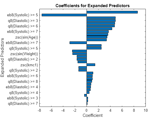
Identify the predictors whose coefficients have larger absolute values.
bigCoefs = abs(sortedCoefs) >= 4;
flip(sortedExpandedPreds(bigCoefs))
ans = 1×7 cell
    {'zsc(Systolic.^2)'}    {'eb8(Systolic) >= 5'}    {'eb8(Diastolic) >= 3'}    {'q8(Diastolic) >= 3'}    {'q8(Systolic) >= 6'}    {'q8(Diastolic) >= 6'}    {'zsc(Height-Systolic)'}
You can use partial dependence plots to analyze the categorical features whose levels have large coefficients in terms of absolute value. For example, inspect the partial dependence plot for the q8(Diastolic) variable, whose levels q8(Diastolic) >= 3 and q8(Diastolic) >= 6 have coefficients with large absolute values. These two levels correspond to noticeable changes in the predicted scores.
plotPartialDependence(Mdl,"q8(Diastolic)",Mdl.ClassNames,NewTbl);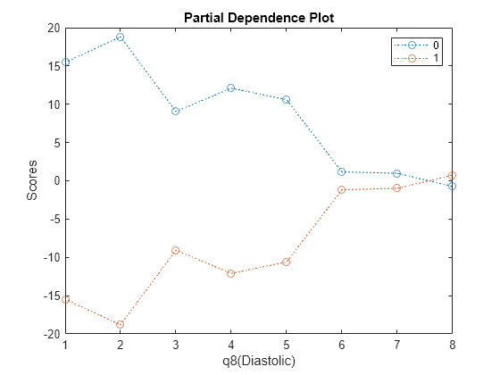
Generate new features to improve the model accuracy for an interpretable linear model. Compare the test set accuracy of a linear model trained on the original data to the test set accuracy of a linear model trained on the transformed features.
Load the ionosphere data set. Convert the matrix of predictors X to a table.
load ionosphere
tbl = array2table(X);
Partition the data into training and test sets. Use approximately 70% of the observations as training data, and 30% of the observations as test data. Partition the data using cvpartition.
rng("default") % For reproducibility of the partition
cvp = cvpartition(Y,Holdout=0.3);

trainIdx = training(cvp);
trainTbl = tbl(training(cvp),:);
trainY = Y(trainIdx);

testIdx = test(cvp);
testTbl = tbl(testIdx,:);
testY = Y(testIdx);
Use the training data to generate 45 new features. Inspect the returned FeatureTransformer object.
[T,newTrainTbl] = gencfeatures(trainTbl,trainY,45);
T
T =
  FeatureTransformer with properties:

                     Type: 'classification'
            TargetLearner: 'linear'
    NumEngineeredFeatures: 45
      NumOriginalFeatures: 0
         TotalNumFeatures: 45
All the generated features are engineered features rather than original features in trainTbl.
Apply the transformations stored in the object T to the test data.
newTestTbl = transform(T,testTbl);
Compare the test set performances of a linear classifier trained on the original features and a linear classifier trained on the new features.
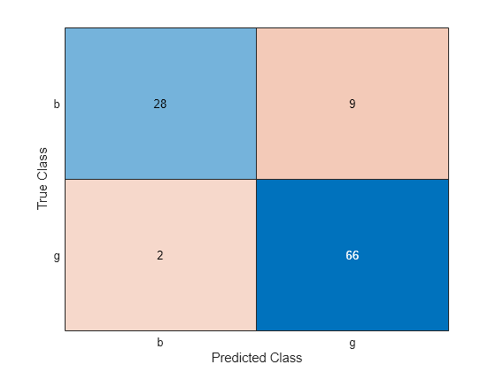
Fit a linear model without transforming the data. Check the test set performance of the model using a confusion matrix.
originalMdl = fitclinear(trainTbl,trainY);
originalPredictedLabels = predict(originalMdl,testTbl);
cm = confusionchart(testY,originalPredictedLabels);
confusionMatrix = cm.NormalizedValues;
originalTestAccuracy = sum(diag(confusionMatrix))/sum(confusionMatrix,"all")
originalTestAccuracy = 0.8952
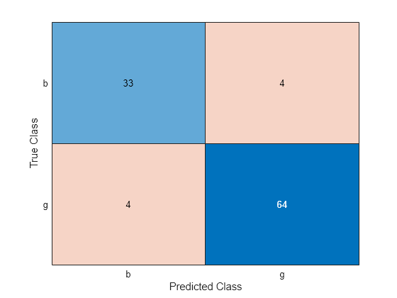
Fit a linear model with the transformed data. Check the test set performance of the model using a confusion matrix.
newMdl = fitclinear(newTrainTbl,trainY);
newPredictedLabels = predict(newMdl,newTestTbl);
newcm = confusionchart(testY,newPredictedLabels);
newConfusionMatrix = newcm.NormalizedValues;
newTestAccuracy = sum(diag(newConfusionMatrix))/sum(newConfusionMatrix,"all")
newTestAccuracy = 0.9143
The linear classifier trained on the transformed data seems to outperform the linear classifier trained on the original data.
Use gencfeatures to engineer new features before training a bagged ensemble classifier. Before making predictions on new data, apply the same feature transformations to the new data set. Compare the test set performance of the ensemble that uses the engineered features to the test set performance of the ensemble that uses the original features.
Read the sample file CreditRating_Historical.dat into a table. The predictor data consists of financial ratios and industry sector information for a list of corporate customers. The response variable consists of credit ratings assigned by a rating agency. Preview the first few rows of the data set.
creditrating = readtable("CreditRating_Historical.dat");
head(creditrating)
ID WC_TA RE_TA EBIT_TA MVE_BVTD S_TA Industry Rating
_____ ______ ______ _______ ________ _____ ________ _______
62394 0.013 0.104 0.036 0.447 0.142 3 {'BB' }
48608 0.232 0.335 0.062 1.969 0.281 8 {'A' }
42444 0.311 0.367 0.074 1.935 0.366 1 {'A' }
48631 0.194 0.263 0.062 1.017 0.228 4 {'BBB'}
43768 0.121 0.413 0.057 3.647 0.466 12 {'AAA'}
39255 -0.117 -0.799 0.01 0.179 0.082 4 {'CCC'}
62236 0.087 0.158 0.049 0.816 0.324 2 {'BBB'}
39354 0.005 0.181 0.034 2.597 0.388 7 {'AA' }
Because each value in the ID variable is a unique customer ID, that is, length(unique(creditrating.ID)) is equal to the number of observations in creditrating, the ID variable is a poor predictor. Remove the ID variable from the table, and convert the Industry variable to a categorical variable.
creditrating = removevars(creditrating,"ID");
creditrating.Industry = categorical(creditrating.Industry);
Convert the Rating response variable to a categorical variable.
creditrating.Rating = categorical(creditrating.Rating, ...
    ["AAA","AA","A","BBB","BB","B","CCC"]);
Partition the data into training and test sets. Use approximately 75% of the observations as training data, and 25% of the observations as test data. Partition the data using cvpartition.
rng("default") % For reproducibility of the partition
c = cvpartition(creditrating.Rating,Holdout=0.25);
trainingIndices = training(c); % Indices for the training set
testIndices = test(c); % Indices for the test set
creditTrain = creditrating(trainingIndices,:);
creditTest = creditrating(testIndices,:);
Use the training data to generate 40 new features to fit a bagged ensemble. By default, the 40 features include original features that can be used as predictors by a bagged ensemble.
[T,newCreditTrain] = gencfeatures(creditTrain,"Rating",40, ...
    TargetLearner="bag");
T
T =
  FeatureTransformer with properties:

                     Type: 'classification'
            TargetLearner: 'bag'
    NumEngineeredFeatures: 34
      NumOriginalFeatures: 6
         TotalNumFeatures: 40
Create newCreditTest by applying the transformations stored in the object T to the test data.
newCreditTest = transform(T,creditTest);
Compare the test set performances of a bagged ensemble trained on the original features and a bagged ensemble trained on the new features.
Train a bagged ensemble using the original training set creditTrain. Compute the accuracy of the model on the original test set creditTest. Visualize the results using a confusion matrix.
originalMdl = fitcensemble(creditTrain,"Rating",Method="Bag");
originalTestAccuracy = 1 - loss(originalMdl,creditTest, ...
    "Rating",LossFun="classiferror")
originalTestAccuracy =
0.7542
predictedTestLabels = predict(originalMdl,creditTest);
confusionchart(creditTest.Rating,predictedTestLabels);
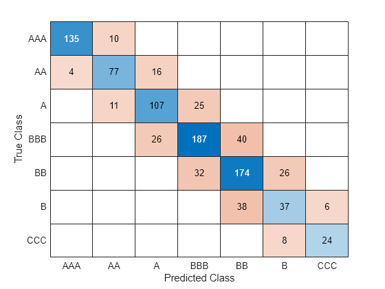
Train a bagged ensemble using the transformed training set newCreditTrain. Compute the accuracy of the model on the transformed test set newCreditTest. Visualize the results using a confusion matrix.
newMdl = fitcensemble(newCreditTrain,"Rating",Method="Bag");
newTestAccuracy = 1 - loss(newMdl,newCreditTest, ...
    "Rating",LossFun="classiferror")
newTestAccuracy =
0.7461
newPredictedTestLabels = predict(newMdl,newCreditTest);
confusionchart(newCreditTest.Rating,newPredictedTestLabels)

The bagged ensemble trained on the transformed data seems to outperform the bagged ensemble trained on the original data.
Engineer and inspect new features before training a binary support vector machine (SVM) classifier with a Gaussian kernel. Then, assess the test set performance of the classifier.
Load the ionosphere data set, which contains radar signal data. The response variable Y indicates the quality of radar returns: g indicates good quality, and b indicates bad quality. Combine the predictor and response data into one table variable.
load ionosphere
Tbl = array2table(X);
Tbl.Y = Y;
head(Tbl)
X1 X2 X3 X4 X5 X6 X7 X8 X9 X10 X11 X12 X13 X14 X15 X16 X17 X18 X19 X20 X21 X22 X23 X24 X25 X26 X27 X28 X29 X30 X31 X32 X33 X34 Y
__ __ _______ ________ ________ ________ ________ ________ _______ ________ _______ ________ _______ ________ ________ ________ ________ ________ ________ ________ ________ ________ ________ ________ ________ ________ ________ ________ ________ ________ ________ ________ ________ ________ _____
1 0 0.99539 -0.05889 0.85243 0.02306 0.83398 -0.37708 1 0.0376 0.85243 -0.17755 0.59755 -0.44945 0.60536 -0.38223 0.84356 -0.38542 0.58212 -0.32192 0.56971 -0.29674 0.36946 -0.47357 0.56811 -0.51171 0.41078 -0.46168 0.21266 -0.3409 0.42267 -0.54487 0.18641 -0.453 {'g'}
1 0 1 -0.18829 0.93035 -0.36156 -0.10868 -0.93597 1 -0.04549 0.50874 -0.67743 0.34432 -0.69707 -0.51685 -0.97515 0.05499 -0.62237 0.33109 -1 -0.13151 -0.453 -0.18056 -0.35734 -0.20332 -0.26569 -0.20468 -0.18401 -0.1904 -0.11593 -0.16626 -0.06288 -0.13738 -0.02447 {'b'}
1 0 1 -0.03365 1 0.00485 1 -0.12062 0.88965 0.01198 0.73082 0.05346 0.85443 0.00827 0.54591 0.00299 0.83775 -0.13644 0.75535 -0.0854 0.70887 -0.27502 0.43385 -0.12062 0.57528 -0.4022 0.58984 -0.22145 0.431 -0.17365 0.60436 -0.2418 0.56045 -0.38238 {'g'}
1 0 1 -0.45161 1 1 0.71216 -1 0 0 0 0 0 0 -1 0.14516 0.54094 -0.3933 -1 -0.54467 -0.69975 1 0 0 1 0.90695 0.51613 1 1 -0.20099 0.25682 1 -0.32382 1 {'b'}
1 0 1 -0.02401 0.9414 0.06531 0.92106 -0.23255 0.77152 -0.16399 0.52798 -0.20275 0.56409 -0.00712 0.34395 -0.27457 0.5294 -0.2178 0.45107 -0.17813 0.05982 -0.35575 0.02309 -0.52879 0.03286 -0.65158 0.1329 -0.53206 0.02431 -0.62197 -0.05707 -0.59573 -0.04608 -0.65697 {'g'}
1 0 0.02337 -0.00592 -0.09924 -0.11949 -0.00763 -0.11824 0.14706 0.06637 0.03786 -0.06302 0 0 -0.04572 -0.1554 -0.00343 -0.10196 -0.11575 -0.05414 0.01838 0.03669 0.01519 0.00888 0.03513 -0.01535 -0.0324 0.09223 -0.07859 0.00732 0 0 -0.00039 0.12011 {'b'}
1 0 0.97588 -0.10602 0.94601 -0.208 0.92806 -0.2835 0.85996 -0.27342 0.79766 -0.47929 0.78225 -0.50764 0.74628 -0.61436 0.57945 -0.68086 0.37852 -0.73641 0.36324 -0.76562 0.31898 -0.79753 0.22792 -0.81634 0.13659 -0.8251 0.04606 -0.82395 -0.04262 -0.81318 -0.13832 -0.80975 {'g'}
0 0 0 0 0 0 1 -1 0 0 -1 -1 0 0 0 0 1 1 -1 -1 0 0 0 0 1 1 1 1 0 0 1 1 0 0 {'b'}
Partition the data into training and test sets. Use approximately 75% of the observations as training data, and 25% of the observations as test data. Partition the data using cvpartition.
rng("default") % For reproducibility of the partition
c = cvpartition(Tbl.Y,Holdout=0.25);
trainTbl = Tbl(training(c),:);
testTbl = Tbl(test(c),:);
Use the training data to generate 50 features to fit a binary SVM classifier with a Gaussian kernel. By default, the 50 features include original features that can be used as predictors by an SVM classifier. Additionally, gencfeatures uses neighborhood component analysis (NCA) to reduce the set of engineered features to the most important predictors. You can use the NCA feature selection method only when the target learner is "gaussian-svm".
[Transformer,newTrainTbl] = gencfeatures(trainTbl,"Y",50, ...
    TargetLearner="gaussian-svm")
Transformer =
  FeatureTransformer with properties:

                     Type: 'classification'
            TargetLearner: 'gaussian-svm'
    NumEngineeredFeatures: 17
      NumOriginalFeatures: 33
         TotalNumFeatures: 50
newTrainTbl=264×51 table
    zsc(X1)    zsc(X3)      zsc(X4)     zsc(X5)    zsc(X6)     zsc(X7)     zsc(X8)     zsc(X9)     zsc(X10)    zsc(X11)     zsc(X12)     zsc(X13)     zsc(X14)      zsc(X15)    zsc(X16)    zsc(X17)    zsc(X18)    zsc(X19)    zsc(X20)     zsc(X21)    zsc(X22)     zsc(X23)     zsc(X24)    zsc(X25)    zsc(X26)    zsc(X27)     zsc(X28)    zsc(X29)    zsc(X30)    zsc(X31)     zsc(X32)     zsc(X33)    zsc(X34)     zsc(X1.*X29)    zsc(X10.*X21)    zsc(X10.*X33)    zsc(X4+X6)    zsc(X5+X6)    zsc(X8+X21)    zsc(X1-X7)    zsc(kmc2)    zsc(kmc6)    q13(X3)    q12(X5)    q15(X6)    q13(X7)    q15(X21)    q14(X27)    eb8(X5)    eb8(X7)      Y
    _______    ________    _________    _______    ________    ________    ________    ________    ________    _________    _________    ________    ___________    ________    ________    ________    ________    ________    _________    ________    _________    _________    ________    ________    ________    _________    ________    ________    ________    ________    __________    ________    _________    ____________    _____________    _____________    __________    __________    ___________    __________    _________    _________    _______    _______    _______    _______    ________    ________    _______    _______    _____

    0.35062     0.71387     -0.24103    0.48341    -0.19017     0.58078     -1.0063     0.97782    -0.26974       0.6391     -0.67348     0.31834        -1.1367     0.38853    -0.98325     0.75294    -0.77965      0.3598     -0.57266     0.38845     -0.60939    -0.012451    -0.80961     0.28949    -0.84597      -0.2517    -0.72759    -0.28242    -0.63852    0.080034       -1.0708    -0.31129       -1.046      -0.26816          0.25043        -0.038585        -0.3418        0.2362       -0.42505      -0.33933       1.0418       1.0355       12         8          7          9           9           6           7          7       {'g'}
    0.35062     0.72301     -0.18451    0.77158    -0.22962     0.91433    -0.49033     0.75792    -0.32357      0.42329     -0.20389     0.73252        -0.1965     0.29679    -0.13823     0.74354    -0.27428     0.64142     -0.10244      0.6146     -0.56742      0.09598    -0.12919     0.30176    -0.62944     0.094562    -0.28922    0.096446    -0.30619        0.41      -0.47923      0.4091      -0.8911       0.14996            0.214        -0.039539        -0.3295       0.42742        0.21888      -0.65367       0.5226      0.75088       13         12         6          13          10          8           8          8       {'g'}
    0.35062     0.72301      -1.1204    0.77158      1.9267     0.33603     -2.2596     -1.0149    -0.34873     -0.87362     -0.31257    -0.64512       -0.21349     -2.0888     0.17363     0.26338    -0.79564     -2.2123      -1.0155     -1.6745       1.8964     -0.63461     0.10334      1.0283      1.9591    -0.047978      1.9396      1.0838    -0.36052    -0.22117        1.9446      -1.294       2.1421        1.2396          0.19008        -0.061281         0.6801        1.8984        -3.5052      -0.10868      -1.5842       -1.337       13         12         15         7           2           7           8          7       {'b'}
    0.35062     -1.2136     -0.12242     -1.375    -0.49905     -1.1101    -0.48554    -0.72188     -0.2093     -0.80643     -0.44067    -0.64512       -0.21349    -0.61619    -0.48568    -0.61727    -0.20429    -0.77473    -0.040295    -0.50751     0.034923     -0.60903     0.12046    -0.62226     0.13548      -1.1087     0.28317     -0.7878    0.053398    -0.68758    -0.0072697    -0.67106      0.21145       -0.8259          0.19351        -0.061365       -0.49849       -1.3813       -0.90111        1.2542      -1.5842       -1.337       3          1          2          2           6           2           4          4       {'b'}
    0.35062     0.67519     -0.34656    0.66615    -0.69083      0.7698    -0.81803     0.69875    -0.92315      0.54191      -1.2868     0.61614        -1.2563     0.60599     -1.4924     0.32568     -1.3793     0.02881      -1.3967    0.052918      -1.5154    -0.097458     -1.4342    -0.29246     -1.4483     -0.78193     -1.3907     -0.5715     -1.5984    -0.76498       -1.5945    -0.93671      -1.8288      -0.58719        -0.089744         0.061186        -0.8284      0.032979       -0.60879      -0.51746       1.0418       1.0355       12         10         1          11          7           4           8          8       {'g'}
    -2.8413     -1.2599     -0.10917    -1.1812    -0.24013     0.91433     -2.2596     -1.0149    -0.34873      -2.6482      -2.3453    -0.64512       -0.21349    -0.54564    -0.14479       1.006      2.0324     -2.2123      -1.9207    -0.53738    -0.035976     -0.63461     0.10334      1.0283      2.1431      0.88773      1.9396    -0.65143    0.038853      1.1285        1.9446    -0.67031    -0.052094       -0.6754          0.19008        -0.061281       -0.27913       -1.0579        -2.3662       -2.5471      -1.5842       -1.337       3          3          6          13          5           14          5          8       {'b'}
    0.35062     0.65074     -0.27034    0.77158     -0.5507     0.91433    -0.67645     0.97782     -1.1087      0.76913      -1.1982     0.87871        -1.0489     0.84926     -1.1622      0.9786    -0.71297     0.78777      -1.2452     0.68706      -1.2068      0.53806     -1.1348     0.77353     -1.1281     0.067353     -1.1572    -0.21008     -1.2312     0.13174       -1.4278    0.078797       -1.663      -0.18832         -0.57784         -0.51689       -0.65574       0.20838        0.14089      -0.65367       1.0418       1.0355       11         12         2          13          10          7           8          8       {'g'}
    0.35062     -1.2969     -0.29857    -1.1812    -0.24013     -1.0948    -0.24765    -0.78637    -0.91197       -1.684      -1.0885    -0.64512       -0.21349      -1.065     0.70198     -1.2124      0.3075     0.44948        0.507    -0.53738    -0.035976     -0.63461     0.10334    -0.93558     0.13961     -0.64684    0.073011    -0.65143    0.038853     -0.3862       0.46286    -0.82839      0.78311       -0.6754          0.19008        0.0099774       -0.42709       -1.0579       -0.73858        1.2397      -1.5842       -1.337       2          3          6          3           5           4           5          5       {'b'}
    0.35062     0.72301     0.039848    0.77158    -0.63857     0.91433    -0.79731     0.97782     -1.2544      0.90098      -1.1531     0.90648        -1.2791     0.85418     -1.4394     0.83179     -1.3466     0.54942      -1.3441     0.61066      -1.5108      0.42766     -1.4494     0.27335     -1.5965      -0.1331     -1.4636    0.047912     -1.6238    -0.12466       -1.7462    -0.22743      -2.0084      0.096399         -0.66792         -0.38227       -0.48436       0.14844      -0.033402      -0.65367       1.0418       1.0355       13         12         1          13          10          7           8          8       {'g'}
    0.35062     0.72301       -1.323    0.77158     -2.4069     0.91433     -2.2596     0.97782     0.41213      0.90098      -1.1484     0.96723         1.8407     0.99753     -2.3384       1.006    -0.59315      1.0392      -1.7935      1.0877       1.8964       1.0494      2.0312      1.0283    -0.64265      0.88773     -1.0301      1.0838     -1.9482      1.1285       -1.9591      1.2557      -2.2463        1.2396           1.2105           1.1115        -2.9765       -1.0579       -0.73858      -0.65367       1.0418       1.0355       13         12         1          13          15          14          8          8       {'b'}
    0.35062     0.72301     0.056082    0.77158    -0.16603     0.91433    -0.35958     0.97782    -0.16462      0.90098     0.086893     0.96723        0.20409     0.99753     0.13566       1.006     0.21703      1.0392      0.60585      1.0877      0.82892       1.0494     0.90821      1.0283     0.56194      0.88773     0.78535      1.0075      1.0054      1.1285       0.62693      1.2557      0.97284        1.1554            0.437          0.22251      -0.090217       0.47081        0.79852      -0.65367       0.5226      0.75088       13         12         8          13          15          14          8          8       {'g'}
    0.35062    -0.24996      -2.2139    0.77158     0.33858     -1.1655     -2.2596     0.97782     -2.4496    -0.098384      -2.3453    -0.64512       -0.21349     -2.0888    -0.89643     -1.2213    0.076204      1.0392      -1.9207    -0.53738    -0.035976     -0.63461     0.10334    -0.96039      1.9896     -0.27735     0.59845    -0.65143    0.038853      1.1285       0.44533    -0.67031    -0.052094       -0.6754          0.19008        -0.061281        -1.4561       0.81505        -2.3662        1.3064      -1.5842       -1.337       5          12         11         2           5           6           8          4       {'b'}
    0.35062     0.71598     0.035661    0.77158    -0.26691     0.87035     -0.1974     0.90034    -0.30016       0.8881     -0.15385     0.79508    -0.00095871     0.90821    -0.02921     0.82498     0.22838     0.81324      0.23893     0.78923      0.19262      0.77433     0.38176     0.70892     0.43102      0.49084     0.36373     0.72129     0.34444     0.71304       0.30366     0.69599      0.21153       0.83955          0.24325       -0.0081697       -0.18761       0.40198        0.63077      -0.61223       0.5226      0.75088       12         12         4          12          11          10          8          8       {'g'}
    0.35062    0.069941    -0.052561    0.11987    -0.13112    0.054366      0.1298    -0.84005     0.36726       0.2554    -0.065971     0.35614       0.079956     0.66786    0.095978      0.3326     0.37109    -0.35253       0.8869     0.33835      0.37612      0.23129     0.53951      0.1531     0.63492     -0.15329     0.56409     0.10222     0.54169    0.050904       0.49615      1.2557      0.67277       0.15634          0.70752           1.0423       -0.14691     0.0012868        0.44389       0.15675       0.5226      0.75088       6          6          8          6           8           6           7          6       {'g'}
    -2.8413     0.72301      -2.3483    -1.1812    -0.24013     -1.0948    -0.24765     0.97782      1.7521      0.90098      -2.3453      -1.804         1.8407    -0.54564    -0.14479     -2.2295      2.0324      1.0392       2.0554     -2.1625       1.8964       1.0494      1.1877      -2.393      2.1431      0.88773      1.9396      1.0838     -1.9482      1.1285        1.9446      1.2557       2.1421       -0.6754          -2.6274           3.1769        -2.0283       -1.0579        -2.3662      -0.65367      0.92994      0.89071       13         3          6          3           1           14          5          5       {'b'}
    -2.8413     0.72301         2.13    -1.1812    -0.24013     -1.0948    -0.24765     -3.0077     -2.4496     -0.87362     -0.31257    -0.64512       -0.21349     -2.0888     -2.3384     -2.2295     -2.0271     -2.2123       2.0554     -2.1625       1.8964     -0.63461     0.10334    -0.68235     0.16583      0.88773     -1.7099     -2.3866      2.0259     -2.5037        1.9446     -2.5963       2.1421       -0.6754           3.0075           3.1769           1.47       -1.0579        -2.3662      -0.65367      -1.5842       -1.337       13         3          6          3           1           14          5          5       {'b'}
      ⋮
By default, gencfeatures standardizes the original features before including them in newTrainTbl. Because it has a constant value of 0, the original X2 variable in trainTbl is not included in newTrainTbl.
unique(trainTbl.X2)
ans =
0
Inspect the first three engineered features. Note that the engineered features are stored after the 33 original features in the Transformer object. Visualize the engineered features by using a matrix of scatter plots and histograms.
featIndex = 34:36;
describe(Transformer,featIndex)
                      Type      IsOriginal    InputVariables                           Transformations
                     _______    __________    ______________    ______________________________________________________________

    zsc(X1.*X29)     Numeric      false          X1, X29        X1 .* X29
                                                                Standardization with z-score (mean = 0.35269, std = 0.5222)
    zsc(X10.*X21)    Numeric      false          X10, X21       X10 .* X21
                                                                Standardization with z-score (mean = -0.067464, std = 0.35493)
    zsc(X10.*X33)    Numeric      false          X10, X33       X10 .* X33
                                                                Standardization with z-score (mean = 0.018924, std = 0.30881)
gplotmatrix(newTrainTbl{:,featIndex},[],newTrainTbl.Y,[], ...
    [],[],[],"grpbars", ...
    newTrainTbl.Properties.VariableNames(featIndex))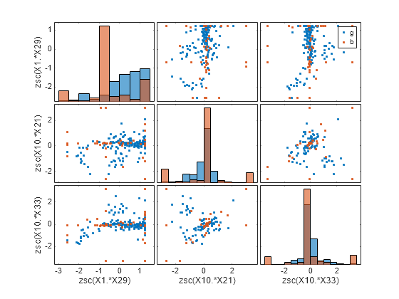
The plots can help you better understand the engineered features. For example:
The top-left plot is a histogram of the
zsc(X1.*X29)feature. This feature consists of the standardized element-wise product of the originalX1andX29features. The histogram shows that the distribution of values corresponding to good radar returns (blue) is different from the distribution of values corresponding to bad radar returns (red). For example, many of the values inzsc(X1.*X29)that correspond to bad radar returns are between –1 and –0.5.The plot in the second row, first column is a scatter plot that compares the
zsc(X1.*X29)values (along the x-axis) to thezsc(X8.*X14)values (along the y-axis). The scatter plot shows that most of thezsc(X8.*X14)values corresponding to good radar returns (blue) are greater than –1, while many of thezsc(X8.*X14)values corresponding to bad radar returns (red) are less than 1. Note that this plot contains the same information as the plot in the first row, second column, but with the axes flipped.
Create newTestTbl by applying the transformations stored in the object Transformer to the test data.
newTestTbl = transform(Transformer,testTbl);
Train an SVM classifier with a Gaussian kernel using the transformed training set newTrainTbl. Let the fitcsvm function find an appropriate scale value for the kernel function. Compute the accuracy of the model on the transformed test set newTestTbl. Visualize the results using a confusion matrix.
Mdl = fitcsvm(newTrainTbl,"Y",KernelFunction="gaussian", ...
    KernelScale="auto");
testAccuracy = 1 - loss(Mdl,newTestTbl,"Y", ...
    LossFun="classiferror")
testAccuracy =
0.9189
predictedTestLabels = predict(Mdl,newTestTbl);
confusionchart(newTestTbl.Y,predictedTestLabels)
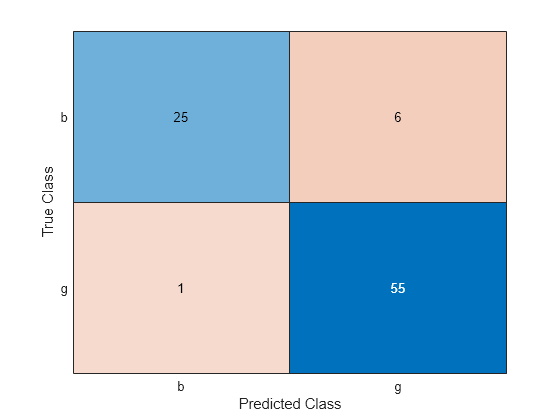
The SVM model correctly classifies most of the observations. That is, for most observations, the class predicted by the SVM model matches the true class label.
Generate features to train a linear classifier. Compute the cross-validation classification error of the model by using the crossval function.
Load the ionosphere data set, and create a table containing the predictor data.
load ionosphere
Tbl = array2table(X);
Create a random partition for stratified 5-fold cross-validation.
rng("default") % For reproducibility of the partition
cvp = cvpartition(Y,KFold=5);
Compute the cross-validation classification loss for a linear model trained on the original features in Tbl.
CVMdl = fitclinear(Tbl,Y,CVPartition=cvp);
cvloss = kfoldLoss(CVMdl)
cvloss =
0.1339
Create the custom function myloss (shown at the end of this example). This function generates 20 features from the training data, and then applies the same training set transformations to the test data. The function then fits a linear classifier to the training data and computes the test set loss.
Note: If you use the live script file for this example, the myloss function is already included at the end of the file. Otherwise, you need to create this function at the end of your .m file or add it as a file on the MATLAB® path.
Compute the cross-validation classification loss for a linear model trained on features generated from the predictors in Tbl.
newcvloss = mean(crossval(@myloss,Tbl,Y,Partition=cvp))
newcvloss =
0.0657
function testloss = myloss(TrainTbl,trainY,TestTbl,testY)
[Transformer,NewTrainTbl] = gencfeatures(TrainTbl,trainY,20);
NewTestTbl = transform(Transformer,TestTbl);
Mdl = fitclinear(NewTrainTbl,trainY);
testloss = loss(Mdl,NewTestTbl,testY, ...
    LossFun="classiferror");
end
Input Arguments
Original features, specified as a table. Each row of Tbl
corresponds to one observation, and each column corresponds to one predictor variable.
Optionally, Tbl can contain one additional column for the response
variable. Multicolumn variables and cell arrays other than cell arrays of character
vectors are not allowed, but datetime, duration,
and various int predictor variables are allowed.
If
Tblcontains the response variable, and you want to create new features from any of the remaining variables inTbl, then specify the response variable by usingResponseVarName.If
Tblcontains the response variable, and you want to create new features from only a subset of the remaining variables inTbl, then specify a formula by usingformula.If
Tbldoes not contain the response variable, then specify a response variable by usingY. The length of the response variable and the number of rows inTblmust be equal.
Data Types: table
Response variable name, specified as the name of a variable in
Tbl.
You must specify ResponseVarName as a character vector or
string scalar. For example, if the response variable Y is stored as
Tbl.Y, then specify it as 'Y'. Otherwise, the
software treats all columns of Tbl as predictors, and might create
new features from Y.
Data Types: char | string
Number of features, specified as a positive integer scalar. For example, you can set
q to approximately 1.5*size(Tbl,2), which is
about 1.5 times the number of original features.
Data Types: single | double
Response variable with observations in rows, specified as a numeric vector, logical
vector, string array, cell array of character vectors, or categorical vector.
Y and Tbl must have the same number of
rows.
Data Types: single | double | logical | string | cell | categorical
Explanatory model of the response variable and a subset of the predictor variables,
specified as a character vector or string scalar in the form
"Y~X1+X2+X3". In this form, Y represents the
response variable, and X1, X2, and
X3 represent the predictor variables.
To create new features from only a subset of the predictor variables in
Tbl, use a formula. If you specify a formula, then the software
does not create new features from any variables in Tbl that do not
appear in formula.
The variable names in the formula must be both variable names in Tbl
(Tbl.Properties.VariableNames) and valid MATLAB® identifiers. You can verify the variable names in Tbl by
using the isvarname function. If the variable names
are not valid, then you can convert them by using the matlab.lang.makeValidName function.
Data Types: char | string
Name-Value Arguments
Specify optional pairs of arguments as
Name1=Value1,...,NameN=ValueN, where Name is
the argument name and Value is the corresponding value.
Name-value arguments must appear after other arguments, but the order of the
pairs does not matter.
Example: gencfeatures(Tbl,"Response",10,TargetLearner="bag",FeatureSelection="oob")
specifies that the expected learner type is a bagged ensemble classifier and the method for
selecting features is an out-of-bag, predictor importance technique.
Expected learner type, specified as "linear",
"bag", or "gaussian-svm". The software creates
and selects new features assuming they will be used to train this type of
model.
| Value | Expected Model |
|---|---|
"linear" | ClassificationLinear — Appropriate
for binary classification only. You can create a model by using the
fitclinear function. |
"bag" | ClassificationBaggedEnsemble —
Appropriate for binary and multiclass classification. You can create a model
by using the fitcensemble function and specifying
Method="Bag". |
"gaussian-svm" | ClassificationSVM (with a Gaussian
kernel) — Appropriate for binary classification only. You can create a model
by using the fitcsvm function and specifying
KernelFunction="gaussian". To create a model with good
predictive performance, specify
KernelScale="auto". |
By default, TargetLearner is "linear",
which supports binary response variables only. If you have a multiclass response
variable and you want to generate new features, you must set
TargetLearner to "bag".
Example: TargetLearner="bag"
Method for including the original features in Tbl in the new
table NewTbl, specified as one of the values in this
table.
| Value | Description |
|---|---|
"auto" | This value is equivalent to:
|
"include" | The software includes original features that can be used as predictors by the target learner, and excludes features that are:
|
"select" | The software includes original features that are supported by the
target learner and considered to be important by the specified feature
selection method (FeatureSelectionMethod). |
"omit" | The software omits the original features. |
Note that the software applies the standardization method specified by the
TransformedDataStandardization name-value argument to original
features included in NewTbl.
Example: IncludeInputVariables="include"
Method for selecting new features, specified as one of the values in this table.
The software generates many features using various transformations and uses this
method to select the important features to include in
NewTbl.
| Value | Description |
|---|---|
"auto" | This value is equivalent to:
|
"lasso" | Lasso regularization — Available when
To perform feature selection, the
software uses |
"oob" | Out-of-bag, predictor importance estimates by permutation —
Available when To perform feature selection, the
software fits a bagged ensemble of trees and uses the |
"nca" | Neighborhood component analysis (NCA) — Available when
To perform feature
selection, the software uses To use
|
"mrmr" | Minimum redundancy maximum relevance (MRMR) — Available when
To perform feature
selection, the software uses |
For more information on different feature selection methods, see Introduction to Feature Selection.
Example: FeatureSelection="mrmr"
Standardization method for the transformed data, specified as one of the values in this table. The software applies this standardization method to both engineered features and original features.
| Value | Description |
|---|---|
"auto" | This value is equivalent to:
|
"zscore" | Center and scale to have mean 0 and standard deviation 1 |
"none" | Use raw data |
"mad" | Center and scale to have median 0 and median absolute deviation 1 |
"range" | Scale range of data to [0,1] |
Example: TransformedDataStandardization="range"
Maximum number of categories allowed in a categorical predictor, specified as a
nonnegative integer scalar. If a categorical predictor has more than the specified
number of categories, then gencfeatures does not create new
features from the predictor and excludes the predictor from the new table
NewTbl. The default value is 50 when
TargetLearner is "linear" or
"gaussian-svm", and Inf when
TargetLearner is "bag".
Example: CategoricalEncodingLimit=20
Data Types: single | double
Output Arguments
Engineered feature transformer, returned as a FeatureTransformer object. To better understand the engineered features, use
the describe
object function of Transformer. To apply the same feature
transformations on a new data set, use the transform
object function of Transformer.
Generated features, returned as a table. Each row corresponds to an observation, and
each column corresponds to a generated feature. If the response variable is included in
Tbl, then NewTbl also includes the response
variable. Use this table to train a classification model of type
TargetLearner.
NewTbl contains generated features in the following order:
original features, engineered features as ranked by the feature selection method, and
the response variable.
Tips
By default, when
TargetLearneris"linear"or"gaussian-svm", the software generates new features from numeric predictors by using z-scores (seeTransformedDataStandardization). You can change the type of standardization for the transformed features. However, using some method of standardization, thereby avoiding the"none"specification, is strongly recommended. Fitting linear and SVM models works best with standardized data.When you generate features to create an SVM model with good predictive performance, specify
KernelScaleas"auto"in the call tofitcsvm. This specification allows the software to find an appropriate scale value for the SVM kernel function.
Version History
Introduced in R2021aWhen the TargetLearner is "linear" or
"gaussian-svm", the gencfeatures function always
excludes original features that are categorical and include missing values, even when
IncludeInputVariables is specified as "include".
That is, the features are not included in the table of generated features
NewTbl. Additionally, gencfeatures does not
generate features from these categorical features with missing values.
To include the original categorical features with missing values in
NewTbl, you can first remove the observations with missing values
from Tbl by using the rmmissing function.
Before training an SVM model with a Gaussian kernel, you can engineer new features from
a data set that contains a mix of numeric and categorical predictors, and use neighborhood
component analysis (NCA) as the method for selecting new features
(FeatureSelectionMethod="nca"). Specify
TargetLearner as "gaussian-svm" in the call to
gencfeatures.
In previous releases, the NCA feature selection method was available for data sets with numeric predictors only.
When the TargetLearner is "linear" or
"gaussian-svm", the gencfeatures function always
excludes original features that include NaN or Inf
values, even when IncludeInputVariables is specified as
"include". That is, the features are not included in the table of
generated features NewTbl. Additionally,
gencfeatures does not generate features from the original features
that include NaN values.
To include the original features with NaN values in
NewTbl, you can first remove the observations with missing values
from Tbl by using the rmmissing function.
MATLAB Command
You clicked a link that corresponds to this MATLAB command:
Run the command by entering it in the MATLAB Command Window. Web browsers do not support MATLAB commands.
Select a Web Site
Choose a web site to get translated content where available and see local events and offers. Based on your location, we recommend that you select: .
You can also select a web site from the following list
How to Get Best Site Performance
Select the China site (in Chinese or English) for best site performance. Other MathWorks country sites are not optimized for visits from your location.
Americas
- América Latina (Español)
- Canada (English)
- United States (English)
Europe
- Belgium (English)
- Denmark (English)
- Deutschland (Deutsch)
- España (Español)
- Finland (English)
- France (Français)
- Ireland (English)
- Italia (Italiano)
- Luxembourg (English)
- Netherlands (English)
- Norway (English)
- Österreich (Deutsch)
- Portugal (English)
- Sweden (English)
- Switzerland
- United Kingdom (English)