invfreqs

R2026b

Identify continuous-time filter parameters from frequency response data

Syntax

[b,a] = invfreqs(h,w,n,m)

[b,a] = invfreqs(h,w,n,m,wt)

[b,a] = invfreqs(h,w,n,m,wt,iter)

[b,a] = invfreqs(h,w,n,m,wt,iter,tol)

[b,a] = invfreqs(h,w,n,m,wt,iter,tol,"trace")

[b,a] = invfreqs(h,w,"complex",n,m,___)

Description

[b,a] = invfreqs(h,w,n,m) returns the real numerator and denominator coefficient vectors b and a of the transfer function h.

[b,a] = invfreqs(h,w,n,m,wt) weights the fit-errors versus frequency using wt.

[b,a] = invfreqs(h,w,n,m,wt,iter) provides an algorithm that guarantees stability of the resulting linear system by searching for the best fit using a numerical, iterative scheme.

[b,a] = invfreqs(h,w,n,m,wt,iter,tol) uses tol to decide convergence of the iterative algorithm.

[b,a] = invfreqs(h,w,n,m,wt,iter,tol,"trace") displays a textual progress report of the iteration. For more information, see Algorithms.

[b,a] = invfreqs(h,w,"complex",n,m,___) creates a complex filter. In this case no symmetry is enforced, and the frequency is specified between –π and π radians per sample. This syntax can include any combination of wt,iter,tol, and "trace" input arguments from the previous syntaxes.

Examples

Transfer Function to Frequency Response Conversion

Convert a simple transfer function to frequency-response data and then back to the original filter coefficients.

a = [1 2 3 2 1 4];
b = [1 2 3 2 3];

[h,w] = freqs(b,a,64);
[bb,aa] = invfreqs(h,w,4,5)

bb = 1×5

    1.0000    2.0000    3.0000    2.0000    3.0000

aa = 1×6

    1.0000    2.0000    3.0000    2.0000    1.0000    4.0000

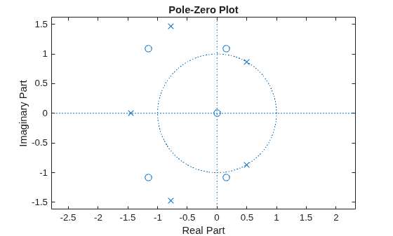
bb and aa are equivalent to b and a, respectively. However, the system is unstable because aa has poles with positive real part. View the poles of bb and aa.

zplane(bb,aa)

Use the iterative algorithm of invfreqs to find a stable approximation to the system.

[bbb,aaa] = invfreqs(h,w,4,5,[],30)

bbb = 1×5

    0.7485    2.2246    3.2889    4.7671   -0.2494

aaa = 1×6

    1.0000    3.2983    7.8655    9.6639    9.3641    0.0004

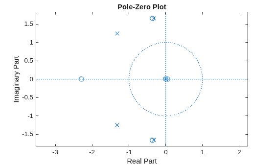
Verify that the system is stable by plotting the new poles.

zplane(bbb,aaa)

Continuous-Time Transfer Function

Generate two vectors, mag and phase, that simulate magnitude and phase data gathered in a laboratory. Also generate a vector, w, of frequencies.

rng('default')

fs = 1000;
t = 0:1/fs:2;
mag = periodogram(sin(2*pi*100*t)+randn(size(t))/10,[],[],fs);
phase = randn(size(mag))/10;
w = linspace(0,fs/2,length(mag))';

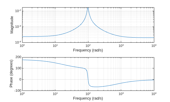
Use invfreqs to convert the data into a continuous-time transfer function. Plot the result.

[b,a] = invfreqs(mag.*exp(1j*phase),w,2,2,[],4);

freqs(b,a)

Input Arguments

h — Frequency response

vector

Frequency response, specified as a vector.

Data Types: single | double

w — Angular frequencies

vector

Angular frequencies at which h is computed, specified as a vector.

n, m — Desired order

positive integer scalar

Desired order of the numerator and denominator polynomials, specified as positive integer scalars.

Data Types: single | double

wt — Weighting factors

vector

Weighting factors, specified as a vector. wt is a vector of weighting factors that is the same length as w.

Data Types: single | double

iter — Number of iterations in the search algorithm

30 (default) | positive real scalar

Number of iterations in the search algorithm, specified as a positive real scalar. The iter parameter tells invfreqs to end the iteration when the algorithm has converged to a solution, or after iter iterations, whichever occurs first.

tol — Tolerance

0.01 (default) | scalar

Tolerance, specified as a scalar. invfreqs defines convergence as occurring when the norm of the (modified) gradient vector is less than tol.

To obtain a weight vector of all ones, use

invfreqs(h,w,n,m,[],iter,tol)

Output Arguments

b, a — Transfer function coefficients

vectors

Transfer function coefficients, returned as vectors. Express the transfer function in terms of b and a as

$$H(s)=\frac{B(s)}{A(s)}=\frac{b(1)s^n+b(2)s^{n-1}+\cdots +b(n+1)}{a(1)s^m+a(2)s^{m-1}+\cdots +a(m+1)}$$

Example: b = [1 3 3 1]/6 and a = [3 0 1 0]/3 specify a third-order Butterworth filter with normalized 3 dB frequency 0.5π rad/sample.

Data Types: double | single
Complex Number Support: Yes

Tips

When building higher order models using high frequencies, it is important to scale the frequencies, dividing by a factor such as half the highest frequency present in w, so as to obtain well-conditioned values of a and b. This corresponds to a rescaling of time.

Algorithms

By default, invfreqs uses an equation error method to identify the best model from the data. The method finds b and a in

$$\underset{a,b}{\arg \min }{\displaystyle \sum _{k=1}^n{W}_{\text{t}}(k){\left|h(k)A(\omega (k))-B(\omega (k))\right|}^2}$$

by creating a system of linear equations and solving them with the MATLAB^® \ operator, where:

• A(ω(k)) and B(ω(k)) are the Fourier transforms of the polynomials a and b, respectively, at the frequency ω(k).

• h(k) is the frequency response at the frequency ω(k).

• W_t(k) contains the weighting factor for the k^th frequency.

• n is the number of frequency points (the length of h, ω, and W_t).

This algorithm is based on Levi [1]. Several variants have been suggested in the literature, where the weighting function W_t gives less importance to high frequencies.

The superior output-error algorithm uses the damped Gauss-Newton method for iterative search [2], with the output of the first algorithm as the initial estimate. The algorithm then solves the direct problem of minimizing the weighted squared 2-norm between the desired frequency response and the response obtained with the estimated coefficients (estimated frequency response).

$$\underset{a,b}{\arg \min }{\Vert \sqrt{W_{\text{t}}(k)}\left[h(k)-\frac{B(\omega (k))}{A(\omega (k))}\right]\Vert }^2$$

The search stops at the end of the iter^th iteration, once the 2-norm of the modified gradient vector is less than tol, or when the 2-norm of the modified gradient vector does not reduce further, whichever occurs first.

If you specify the "trace" argument, the function prints the estimation progress per iteration in the MATLAB command window. For each iteration, invfreqs prints this information:

• Fit accuracy — Squared 2-norm between the desired and estimated frequency responses. The Current Fit and Previous Fit terms list the squared 2-norm associated with the current and previous iteration, respectively.

• Filter coefficient estimates — Three-column matrix, where each column lists this information:

  • Current par is the vector of estimated filter coefficients for the current iteration.

  • prev. par is the vector of estimated filter coefficients for the previous iteration.

  • GN-dir is the modified gradient vector from the Gauss-Newton optimization applied to the current iteration.

  The function lists the vectors of estimated filter coefficients as [α₁; α₂; ⋯; α_m; β₁; β₂; ⋯; β_n+1], where

  $$h(s)=\frac{{\beta }_1{s}^n+{\beta }_2{s}^{n-1}+\cdots +{\beta }_{n+1}}{s^m+{\alpha }_1{s}^{m-1}+{\alpha }_2{s}^{m-2}+\cdots +{\alpha }_m}$$.

• Norm of the Gauss-Newton optimization vector — The Norm of GN-vector lists the 2-norm of the modified gradient vector GN-dir.

References

[1] Levi, E. C. “Complex-Curve Fitting.” IRE Transactions on Automatic Control. Vol. AC-4, 1959, pp. 37–44.

[2] Dennis, J. E., Jr., and R. B. Schnabel. Numerical Methods for Unconstrained Optimization and Nonlinear Equations. Englewood Cliffs, NJ: Prentice-Hall, 1983.

Extended Capabilities

C/C++ Code Generation
Generate C and C++ code using MATLAB® Coder™.

GPU Code Generation
Generate CUDA® code for NVIDIA® GPUs using GPU Coder™.

Thread-Based Environment

Run code in the background using MATLAB® backgroundPool or accelerate code with Parallel Computing Toolbox™ ThreadPool.

The invfreqs function fully supports thread-based environments. For more information, see Run MATLAB Functions in Thread-Based Environment.

Version History

Introduced before R2006a

R2026b: Use thread-based environments

You can use invfreqs in thread-based environments. For more information, see Run MATLAB Functions in Thread-Based Environment.

R2024b: invfreqs supports C/C++ code generation

The invfreqs function supports C/C++ code generation. You must have MATLAB Coder™ to use this functionality.