Wide-band Band Pass filter using a Cascade of High Pass and Low Pass Filter
In this example high pass and low pass filters are created using the filterStub and filterStepImpedanceLowPass catalog itmas and combined using the pcbcascade functionality to give the cascaded filter layout. The cascaded filter layout is solved using the full wave MOM Solver. The filter is designed to exhibit a passband between 3 GHz to 6 GHz.
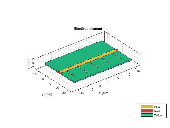
Use the filterStub to create the stub object and change the properties of the filter as given below to create a high pass filter with five stubs. These values can be modified to shift the cut off frequency of the filter. This catalog offers flexibility to create any filter which has any number of stubs with different length, width and position. Use the show function to visualize the filter geometry.
HPF = filterStub;
HPF.PortLineLength = 3e-3;
HPF.PortLineWidth = 1.6e-3;
HPF.SeriesLineWidth = 1.8e-3;
HPF.SeriesLineLength = 24.28e-3;
HPF.StubLength = [6.35e-3 6.35e-3 6.35e-3 6.35e-3 6.35e-3]*1.2;
HPF.StubWidth = [0.238e-3 0.238e-3 0.238e-3 0.238e-3 0.238e-3];
HPF.StubOffsetX = [-2*6.07e-3 -6.07e-3 0 6.07e-3 2*6.07e-3];
HPF.StubShort = [0 0 0 0 0];
HPF.StubDirection = [0 0 0 0 0];
HPF.Height = 0.508e-3;
HPF.StubShort = [1 1 1 1 1];
figure,show(HPF);
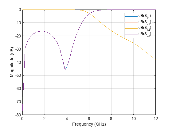
Use the sparameters function to calculate the s-parameters of the high pass filter and plot them using rfplot. The cut off frequency for the High Pass Filter is about 3 GHz.
FreqRange = linspace(1e6,12e9,51);
sparHPF = sparameters(HPF,FreqRange);
figure,rfplot(sparHPF);

Use the filterStepImpedanceLowPass filter to create a low pass filter.
LPF = filterStepImpedanceLowPass;
LPF.Substrate = dielectric('Teflon');
LPF.Height = 0.508e-3;
LPF.FilterOrder = 7;
Use the design function to design the filter with a cut off frequency of 7 GHz. The Cut off frequency is chosen to be silghtly more than the required bandwidth, as there will be some mismatch between the designed and the simulated result. Visualize the geometry using show function.
LPF = design(LPF,7e9);
LPF.PortLineLength = 3e-3;
LPF.PortLineWidth = HPF.PortLineWidth;
figure,show(LPF);

Use sparameters function to calculate the s-parameters and plot them using rfplot function..
sparLPF = sparameters(LPF,FreqRange);
figure,rfplot(sparLPF) ;
Use the pcbcascade functionality to cascade the LowPass and High Pass filter objects. The RectangularBoard can be set to true or false depending on the requirement, where a true value will create the rectangular dielectric board shape. Visualize the geometry using the show function.
BPF = pcbcascade(LPF,HPF,"RectangularBoard",true);
figure,show(BPF);
Use the mesh function to manually mesh the structure,
figure,mesh(BPF,"MaxEdgeLength",2e-3)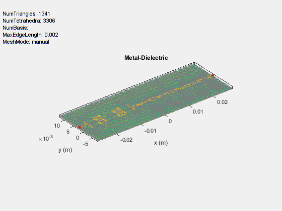
Use the sparameters function to calculate the s-parameters of the cascaded filters and plot them using rfplot. Observe that we obtain a filter passband that is the intersection of the high pass and low pass.
sparBPF = sparameters(BPF,FreqRange);
figure,rfplot(sparBPF);

% s21_MoM = 20*log10(abs(rfparam(sparBPF,2,1)));Using this procedure any high pass and low pass filter can be used to create a band pass response with required Bandwidth. If the pass bands are not overlapping then a band stop filter will be created.
The band pass filter can also be simulated using an FEM Solver and for this the IsShielded property needs to be enabled. Set the IsShielded Property to 1 to enable the metal shield and simulate using FEM Solver
% BPF.IsShielded = 1;
% sparBPF_FEM = sparameters(BPF,FreqRange);
% figure,rfplot(sparBPF_FEM);
%
% s21_FEM = 20*log10(rfparam(sparBPF_FEM,2,1));
% figure,plot(sparBPF.Frequencies,s21_MoM,"LineWidth",2);
% hold on
% plot(sparBPF.Frequencies,s21_FEM,"LineWidth",2);
% hold off
% legend('S21 MoM','S21 FEM');
You can also select a web site from the following list:
Americas
- América Latina (Español)
- Canada (English)
- United States (English)
Europe
- Belgium (English)
- Denmark (English)
- Deutschland (Deutsch)
- España (Español)
- Finland (English)
- France (Français)
- Ireland (English)
- Italia (Italiano)
- Luxembourg (English)
- Netherlands (English)
- Norway (English)
- Österreich (Deutsch)
- Portugal (English)
- Sweden (English)
- Switzerland
- United Kingdom (English)