Design and Optimization of Hairpin Filter using Pattern Search

Step 1 of 4 in Microstrip Band-pass filter based RF Filter Bank for microwave applications

In this example, a hairpin filter is designed and optimized to achieve the required transmission s-parameters. The input response is given to the patternSearch optimizer so that the hairpin filter is optimized to generate that response for S21.

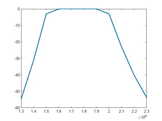
Input Response for Optimizer

Generate an ideal response for a bandpass filter using the rffilter object available in RF Toolbox. This response will be given as input to the optimizer and the optimization will be run taking this as the goal to be achieved. Extract the S21 from the sparameters object using the rfparam function.

filt = rffilter("ResponseType","Bandpass","PassbandFrequency",[1.5e9 2e9],"StopbandAttenuation",40,"StopbandFrequency",[0.8e9 2.2e9]);
data=sparameters(filt,linspace(1.3e9,2.3e9,11));
s21 = 20*log10(abs(rfparam(data,2,1)));
figure,plot(data.Frequencies,s21,"LineWidth",2);

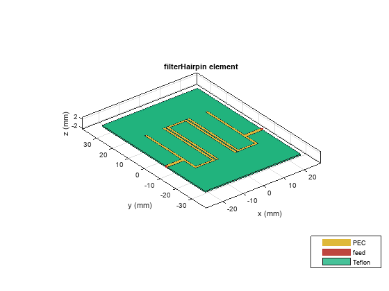
Design Hairpin Filter

Change the Substrate height to 0.508e-3 and use the design function to design the filterHairpin at the center frequency of 1.75 GHz.

freq = data.Frequencies;
Z0 = 50;
pcb = filterHairpin;
pcb.Height = 0.508e-3;
pcb = design(pcb,sum(filt.PassbandFrequency)/2,'Z0',Z0);
pcb.PortLineWidth = 1.6e-3;

Visualize the geometry using the show function.

figure,show(pcb);

Use the sparameters function to compute the s-parameters and plot them using the rfplot function. Observe that the bandwidth obtained is very narrow, about 60 MHz .

spar = sparameters(pcb,linspace(1.3e9,2.4e9,61));
figure,rfplot(spar);

Initial Parameter values

Setup the parameters which will be used in the optimization and add the Lower Bounds and Upper Bounds. For this optimization Resonator Length, Width and Offset, Feed Offset and Spacing between the resonators are taken as optimization parameters.

initial_values = [pcb.Resonator.Length,pcb.Resonator.Width,pcb.ResonatorOffset,pcb.FeedOffset,pcb.Spacing];                 
LB = [25e-3 3e-3 25e-3 0.4e-3 0.4e-3 0.4e-3 -5e-3 -5e-3 -5e-3 -10e-3 -10e-3 0.4e-3 0.4e-3];
UB = [35e-3 15e-3 35e-3 4e-3 4e-3 4e-3 6e-3 6e-3 6e-3 8e-3 8e-3 2e-3 2e-3];
constraints.S21 = s21;

Optimization Parameters

Use the optimoptions to setup the parameters required for the patternsearch optimization with maximum iterations set to 250.

optimizerparams = optimoptions(@patternsearch);
optimizerparams.UseCompletePoll = true;    
optimizerparams.UseCompleteSearch = true;
optimizerparams.PlotFcns = @psplotbestf;
optimizerparams.UseParallel = canUseGPU();
optimizerparams.Cache = "on";
optimizerparams.MaxIter = 250;
optimizerparams.FunctionTolerance = 1e-4;
optimizerOptions = optimizerparams;

Run the patternsearch Optimization on the Objective Function of Hairpin filter with the initial values, lower and upper bound and the optimizer options that are already set. The objective function will compare the S21 obtained by solving the hairpin filter with the Input response that is given to it and provides the result which closely matches that of the Input Response. The objective function is written in such a way that it will give more weight to the pass band response, because it is required to be matched to the input response over the stop band.

[optimpcb] = patternsearch(@(x) Objective_WaveformInputOptimization(pcb,x,freq,filt.PassbandFrequency,...
                                        Z0,constraints),initial_values,[],...
                                    [],[],[],LB,UB,[],optimizerOptions);

patternsearch stopped by the output or plot function.

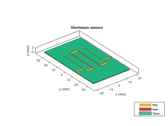
Optimized properties

Assign the updated property values obtained from the optimization and visualize the geometry.using the show function.

optipcb = copy(pcb);
optipcb.Resonator.Length = optimpcb(1:3);
optipcb.Resonator.Width = optimpcb(4:6);
optipcb.ResonatorOffset = optimpcb(7:9);
optipcb.FeedOffset = optimpcb(10:11);
optipcb.Spacing = optimpcb(12:13);
figure,show(optipcb);

Use the sparameters function to plot the s-parameters. The result comparison, before and after the optimization, is plotted using sparameters.

spar = sparameters(optipcb,linspace(1.3e9,2.4e9,61));
figure,rfplot(spar);

The result shows the Bandwidth of the filter is improved to about 350 MHz, and the pass band shifts towards the required response.Using this precedure any item in RF PCB Toolbox filter catalog can be used to design and optimized a filter.

Microstrip Band-pass filter based RF Filter Bank for microwave applications

Next