Design and Optimization of Coupled Line Filter using Surrogate Opt method
In this example, a coupled line filter is designed at 2.5 GHz and the optimization is run on that structure to improve the required bandWidth with constraints on the return loss and insertion Loss. The Objective function is written to Improve both S21 and S11, and the function value is minimized to get an improved return loss and insertion loss.
Use the design function to design the filterCoupledLine at 2,5 GHz and visualize it using the show method.
freq = 2.5e9;
Z0 = 50;
BW = 1e9;
pcb = filterCoupledLine;
pcb.Height = 0.508e-3;
pcb = design(pcb,freq,'Z0',Z0,'FBW',30);
pcb.PortLineLength = 4e-3;
figure,show(pcb);

Use the sparameters method to calculate the s-parameters and plot them using the rfplot function.
spar = sparameters(pcb,linspace(1.5e9,3.5e9,101));
figure,rfplot(spar);
Initial Parameter values
To setup the optimization problem, we need to give the parameters in the geometry which need to be used in the optimization. We will use the CoupledLineLength, CoupledLineWidth and CoupledLineSpacing properties of the filterCoupledLine, but sdditional properties can be added to the optimization. Create the lower and upper bounds for those properties as shown below.
initial_values = [pcb.CoupledLineLength,pcb.CoupledLineWidth,pcb.CoupledLineSpacing];
LB = initial_values*0.6;
UB = initial_values*1.4;

constraints.S11min = -40;
constraints.S12max = -0.5;
Optimization Parameters
Use the optimization to setup the options for the surrogate optimizer and set the UseParallel to true and MaxIterations to 600.
optimizerparams = optimoptions(@surrogateopt);
optimizerparams.UseParallel = true;
optimizerparams.MaxFunctionEvaluations = 600;
optimizerparams.MinSurrogatePoints = 20;
optimizerparams.InitialPoints = initial_values;
Run the surrogateopt Optimization on the Objective Function of coupled line filter with the initial values, lower and upper bound and the optimizer options that we have initialized. The most important step is to assign objectives for the optimization, as the result will depend on the objectives set in the objective function.For this optimization S21 and S11 values are calculated in the passband, and the objective function will minimize the S11 value and maximize the S21 value. The Bandwidth of the optimization is specified as 1 GHz for this optimization.
[optimpcb] = surrogateopt(@(x) Objective_filterCoupledLine(pcb,x,freq,BW,...
                                        Z0,constraints),LB,UB,optimizerparams);
Starting parallel pool (parpool) using the 'Processes' profile ... Connected to parallel pool with 4 workers.
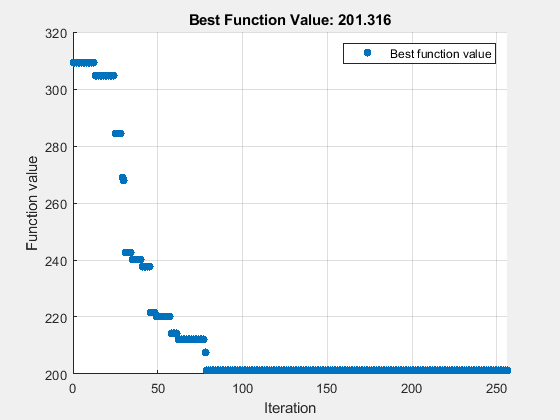
Optimization stopped by a plot function or output function.
Assign the Optimized properties and Run the result
The properties obtained from the optimization are assigned to the object and the filter can be visualized using the show function.
Optipcb = copy(pcb);
Optipcb.CoupledLineLength = optimpcb(1:4);
Optipcb.CoupledLineWidth = optimpcb(5:8);
Optipcb.CoupledLineSpacing = optimpcb(9:12);
figure,show(Optipcb);

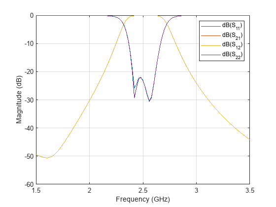
Use the sparameters function to plot the s-parameters for the optimized filter.
spar = sparameters(Optipcb,linspace(1.5e9,3.5e9,101));
figure,rfplot(spar);

The Bandwidth of the Filter is close to 700 MHz which is a improvement of around 300 MHz and the S11 is also improved. In this way any item in the RF PCB Toolbox filter catalog can be used to design and the optimize a filter..
You can also select a web site from the following list
Americas
- América Latina (Español)
- Canada (English)
- United States (English)
Europe
- Belgium (English)
- Denmark (English)
- Deutschland (Deutsch)
- España (Español)
- Finland (English)
- France (Français)
- Ireland (English)
- Italia (Italiano)
- Luxembourg (English)
- Netherlands (English)
- Norway (English)
- Österreich (Deutsch)
- Portugal (English)
- Sweden (English)
- Switzerland
- United Kingdom (English)
Asia Pacific
- Australia (English)
- India (English)
- New Zealand (English)
- 中国
- 日本Japanese (日本語)
- 한국Korean (한국어)