rlPGAgent

Policy gradient (PG) reinforcement learning agent

Description

The policy gradient (PG) algorithm is a on-policy reinforcement learning method for environments with a discrete or continuous action space. A policy gradient agent uses the REINFORCE algorithm to directly estimate a stochastic policy. As REINFORCE belongs to the class of Monte Carlo methods, learning occurs only after an episode is finished. For continuous action spaces, this agent does not enforce constraints set in the action specification; therefore, if you need to enforce action constraints, you must do so within the environment. As this algorithm belongs to the class of Monte Carlo methods, the agent does not learn during an episode but only after an episode is finished.

For more information on PG agents and the REINFORCE algorithm, see REINFORCE Policy Gradient (PG) Agent. For more information on the different types of reinforcement learning agents, see Reinforcement Learning Agents.

Creation

Syntax

agent = rlPGAgent(observationInfo,actionInfo)

agent = rlPGAgent(observationInfo,actionInfo,initOpts)

agent = rlPGAgent(actor)

agent = rlPGAgent(actor,critic)

agent = rlPGAgent(___,agentOptions)

Description

Create Agent from Observation and Action Specifications

agent = rlPGAgent(observationInfo,actionInfo) creates a policy gradient agent for an environment with the given observation and action specifications, using default initialization options. The actor and critic in the agent use default deep neural networks built from the observation specification observationInfo and the action specification actionInfo. The ObservationInfo and ActionInfo properties of agent are set to the observationInfo and actionInfo input arguments, respectively.

agent = rlPGAgent(observationInfo,actionInfo,initOpts) creates a policy gradient agent for an environment with the given observation and action specifications. The agent uses default networks in which each hidden fully connected layer has the number of units specified in the initOpts object. For more information on the initialization options, see rlAgentInitializationOptions.

Create Agent from Actor and Critic

agent = rlPGAgent(actor) creates a policy gradient agent with the specified actor network. By default, the UseBaseline property of the agent is false in this case.

agent = rlPGAgent(actor,critic) creates a policy gradient agent with the specified actor and critic networks. By default, the UseBaseline option is true in this case.

Specify Agent Options

agent = rlPGAgent(___,agentOptions) creates a policy gradient agent and sets the AgentOptions property to the agentOptions input argument. Use this syntax after any of the input arguments in the previous syntaxes.

Input Arguments

initOpts — Agent initialization options

rlAgentInitializationOptions object

Agent initialization options, specified as an rlAgentInitializationOptions object.

actor — Actor

rlDiscreteCategoricalActor object | rlContinuousGaussianActor object

Actor that implements the policy, specified as an rlDiscreteCategoricalActor or rlContinuousGaussianActor function approximator object. For more information on creating actor approximators, see Create Policies and Value Functions.

critic — Baseline critic

rlValueFunction object

Baseline critic that estimates the discounted long-term reward, specified as an rlValueFunction object. For more information on creating critic approximators, see Create Policies and Value Functions.

Properties

ObservationInfo — Observation specifications

specification object | array of specification objects

Observation specifications, specified as an rlFiniteSetSpec or rlNumericSpec object or an array containing a mix of such objects. Each element in the array defines the properties of an environment observation channel, such as its dimensions, data type, and name.

If you create the agent by specifying an actor or critic, the value of ObservationInfo matches the value specified in the actor and critic objects. If you create a default agent, the agent constructor function sets the ObservationInfo property to the input argument observationInfo.

You can extract observationInfo from an existing environment, function approximator, or agent using getObservationInfo. You can also construct the specifications manually using rlFiniteSetSpec or rlNumericSpec.

Example: [rlNumericSpec([2 1]) rlFiniteSetSpec([3,5,7])]

ActionInfo — Action specification

rlFiniteSetSpec object | rlNumericSpec object

Action specifications, specified either as an rlFiniteSetSpec (for discrete action spaces) or rlNumericSpec (for continuous action spaces) object. This object defines the properties of the environment action channel, such as its dimensions, data type, and name.

Note

For this agent, only one action channel is allowed.

If you create the agent by specifying an actor and critic, the value of ActionInfo matches the value specified in the actor and critic objects. If you create a default agent, the agent constructor function sets the ActionInfo property to the input argument ActionInfo.

You can extract actionInfo from an existing environment, function approximator, or agent using getActionInfo. You can also construct the specification manually using rlFiniteSetSpec or rlNumericSpec.

Example: rlNumericSpec([2 1])

AgentOptions — Agent options

rlPGAgentOptions object

Agent options, specified as an rlPGAgentOptions object.

UseExplorationPolicy — Option to use exploration policy for simulation and deployment

true (default) | false

Option to use exploration policy when selecting actions during simulation or after deployment, specified as a one of the following logical values.

• true — Use the base agent exploration policy when selecting actions in sim and generatePolicyFunction. Specifically, in this case the agent uses the rlStochasticActorPolicy policy with the UseMaxLikelihoodAction property set to false. Since the agent selects its actions by sampling its probability distribution, the policy is stochastic and the agent explores its action and observation spaces.

• false — Force the agent to use the base agent greedy policy (the action with maximum likelihood) when selecting actions in sim and generatePolicyFunction. Specifically, in this case the agent uses the rlStochasticActorPolicy policy with the UseMaxLikelihoodAction property set to true. Since the agent selects its actions greedily the policy behaves deterministically and the agent does not explore its action and observation spaces.

Note

This option affects only simulation and deployment; it does not affect training. When you train an agent using train, the agent always uses its exploration policy independently of the value of this property.

SampleTime — Sample time of agent

1 (default) | positive scalar | -1

Sample time of the agent, specified as a positive scalar or as -1.

Within a MATLAB^® environment, the agent is executed every time the environment advances, so, SampleTime does not affect the timing of the agent execution.

Within a Simulink^® environment, the RL Agent block that uses the agent object executes every SampleTime seconds of simulation time. If SampleTime is -1 the block inherits the sample time from its input signals. Set SampleTime to -1 when the block is a child of an event-driven subsystem.

Note

Set SampleTime to a positive scalar when the block is not a child of an event-driven subsystem. Doing so ensures that the block executes at appropriate intervals when input signal sample times change due to model variations.

Regardless of the type of environment, the time interval between consecutive elements in the output experience returned by sim or train is always SampleTime.

If SampleTime is -1, for Simulink environments, the time interval between consecutive elements in the returned output experience reflects the timing of the events that trigger the RL Agent block execution, while for MATLAB environments, this time interval is considered equal to 1.

This property is shared between the agent and the agent options object within the agent. Therefore, if you change it in the agent options object, it gets changed in the agent, and vice versa.

Example: SampleTime=-1

Object Functions

train	Train reinforcement learning agents within a specified environment
sim	Simulate trained reinforcement learning agents within specified environment
getAction	Obtain action from agent, actor, or policy object given environment observations
getActor	Extract actor from reinforcement learning agent
setActor	Set actor of reinforcement learning agent
getCritic	Extract critic from reinforcement learning agent
setCritic	Set critic of reinforcement learning agent
generatePolicyFunction	Generate MATLAB function that evaluates policy of an agent or policy object

Examples

Create Default Policy Gradient Agent

Create an environment and obtain its observation and action specifications. For this example, load the environment used in the example Create DQN Agent Using Deep Network Designer and Train Using Image Observations. This environment has two observations: a 50-by-50 grayscale image and a scalar (the angular velocity of the pendulum). The action is a scalar with five possible elements (a torque of -2, -1, 0, 1, or 2 Nm applied to the pole).

env = rlPredefinedEnv("SimplePendulumWithImage-Discrete");

Obtain observation and action specification objects.

obsInfo = getObservationInfo(env);
actInfo = getActionInfo(env);

The agent creation function initializes the actor and critic networks randomly. Ensure reproducibility by fixing the seed of the random generator.

rng(0)

Create a policy gradient agent from the environment observation and action specifications. Since actInfo is an rlFiniteSetSpec object, rlPGAgent creates an agent with a discrete action space. When actInfo is an rlNumericSpec object, rlPGAgent creates an agent with a continuous action space.

agent = rlPGAgent(obsInfo,actInfo);

To check your agent, use getAction to return the action from a random observation.

getAction(agent,{rand(obsInfo(1).Dimension),rand(obsInfo(2).Dimension)})

ans = 1x1 cell array
    {[-2]}

You can now test and train the agent within the environment.

Create Default Policy Gradient Agent Using Initialization Options

Create an environment and obtain its observation and action specifications. For this example, load the environment used in the example Train DDPG Agent to Swing Up and Balance Pendulum with Image Observation. This environment has two observations: a 50-by-50 grayscale image and a scalar (the angular velocity of the pendulum). The action is a scalar representing a torque ranging continuously from -2 to 2 Nm.

env = rlPredefinedEnv("SimplePendulumWithImage-Continuous");

Obtain observation and action specifications.

obsInfo = getObservationInfo(env);
actInfo = getActionInfo(env);

Create an agent initialization option object, specifying that each hidden fully connected layer in the network must have 128 neurons (instead of the default number, 256). Policy gradient agents do not support recurrent networks, so setting the UseRNN option to true generates an error when the agent is created.

initOpts = rlAgentInitializationOptions(NumHiddenUnit=128);

The agent creation function initializes the actor and critic networks randomly. Ensure reproducibility by fixing the seed of the random generator.

rng(0)

Create a policy gradient agent from the environment observation and action specifications. Since actInfo is an rlNumericSpec object, rlPGAgent creates an agent with a continuous action space. When actInfo is an rlFiniteSetSpec object, rlPGAgent creates an agent with a discrete action space.

agent = rlPGAgent(obsInfo,actInfo,initOpts);

Extract the deep neural networks from both the agent actor and critic.

actorNet = getModel(getActor(agent));
criticNet = getModel(getCritic(agent));

To verify that each hidden fully connected layer has 128 neurons, you can display the layers on the MATLAB® command window,

criticNet.Layers

or visualize the structure interactively using analyzeNetwork.

analyzeNetwork(criticNet)

Plot actor and critic networks, and display their number of weights.

plot(actorNet)

summary(actorNet)

   Initialized: true

   Number of learnables: 18.9M

   Inputs:
      1   'input_1'   50x50x1 images
      2   'input_2'   1 features

plot(criticNet)

summary(criticNet)

   Initialized: true

   Number of learnables: 18.9M

   Inputs:
      1   'input_1'   50x50x1 images
      2   'input_2'   1 features

To check your agent, use getAction to return the action from a random observation.

getAction(agent,{rand(obsInfo(1).Dimension),rand(obsInfo(2).Dimension)})

ans = 1x1 cell array
    {[0.9228]}

You can now test and train the agent within the environment.

Create a Discrete PG Agent from Actor and Baseline Critic

Create an environment with a discrete action space, and obtain its observation and action specifications. For this example, load the environment used in the example Train PG Agent with Custom Networks to Control Discrete Double Integrator. The observation from the environment is a vector containing the position and velocity of a mass. The action is a scalar representing a force, applied to the mass, having three possible values (-2, 0, or 2 Newton).

env = rlPredefinedEnv("DoubleIntegrator-Discrete");
obsInfo = getObservationInfo(env)

obsInfo = 
  rlNumericSpec with properties:

     LowerLimit: -Inf
     UpperLimit: Inf
           Name: "states"
    Description: "x, dx"
      Dimension: [2 1]
       DataType: "double"

actInfo = getActionInfo(env)

actInfo = 
  rlFiniteSetSpec with properties:

       Elements: [-2 0 2]
           Name: "force"
    Description: [0x0 string]
      Dimension: [1 1]
       DataType: "double"

Policy-gradient agents can optionally use a parametrized baseline function to approximate the value of the policy. A value-function approximator takes the current observation as input and returns a single scalar as output (the estimated discounted cumulative long-term reward for following the policy from the state corresponding to the current observation).

To model the parametrized baseline function, use a neural network with one input layer (which receives the content of the observation channel, as specified by obsInfo) and one output layer (which returns the scalar value). Note that prod(obsInfo.Dimension) returns the total number of dimensions of the observation space regardless of whether the observation space is a column vector, row vector, or matrix.

Define the network as an array of layer objects.

baselineNet = [
    featureInputLayer(prod(obsInfo.Dimension))
    fullyConnectedLayer(64)
    reluLayer
    fullyConnectedLayer(1)
    ];

Convert to a dlnetwork object, initialize it, and display the number of weights.

baselineNet = dlnetwork(baselineNet);
baselineNet = initialize(baselineNet);
summary(baselineNet)

   Initialized: true

   Number of learnables: 257

   Inputs:
      1   'input'   2 features

Create the baseline approximator object using baselineNet and the observation specification. For more information on value function approximators, see rlValueFunction.

baseline = rlValueFunction(baselineNet,obsInfo);

Check the critic with a random input observation.

getValue(baseline,{rand(obsInfo.Dimension)})

ans = single

-0.1204

Policy gradient agents use a parametrized stochastic policy, which for discrete action spaces is implemented by a discrete categorical actor. This actor takes an observation as input and returns as output a random action sampled (among the finite number of possible actions) from a categorical probability distribution.

To model the parametrized policy within the actor, use a neural network with one input layer (which receives the content of the environment observation channel, as specified by obsInfo) and one output layer. The output layer must return a vector of probabilities for each possible action, as specified by actInfo. Note that numel(actInfo.Dimension) returns the number of elements of the discrete action space.

Define the network as an array of layer objects.

actorNet = [
    featureInputLayer(prod(obsInfo.Dimension))
    fullyConnectedLayer(64)
    reluLayer
    fullyConnectedLayer(numel(actInfo.Elements))
    ];

Convert to a dlnetwork object, initialize it, and display the number of weights.

actorNet = dlnetwork(actorNet);
actorNet = initialize(actorNet);
summary(actorNet)

   Initialized: true

   Number of learnables: 387

   Inputs:
      1   'input'   2 features

Create the actor using actorNet and the observation and action specifications. For more information on discrete categorical actors, see rlDiscreteCategoricalActor.

actor = rlDiscreteCategoricalActor(actorNet,obsInfo,actInfo);

Check the actor with a random observation input.

getAction(actor,{rand(obsInfo.Dimension)})

ans = 1x1 cell array
    {[-2]}

Create the PG agent using the actor and the baseline critic.

agent = rlPGAgent(actor,baseline)

agent = 
  rlPGAgent with properties:

            AgentOptions: [1x1 rl.option.rlPGAgentOptions]
    UseExplorationPolicy: 1
         ObservationInfo: [1x1 rl.util.rlNumericSpec]
              ActionInfo: [1x1 rl.util.rlFiniteSetSpec]
              SampleTime: 1

Specify options for the agent, including training options for the actor and critic.

agent.AgentOptions.UseBaseline = true;
agent.AgentOptions.DiscountFactor = 0.99;
 
agent.AgentOptions.CriticOptimizerOptions.LearnRate = 5e-3;
agent.AgentOptions.CriticOptimizerOptions.GradientThreshold = 1;
 
agent.AgentOptions.ActorOptimizerOptions.LearnRate = 5e-3;
agent.AgentOptions.ActorOptimizerOptions.GradientThreshold = 1;

Check the agent with a random observation input.

getAction(agent,{rand(obsInfo.Dimension)})

ans = 1x1 cell array
    {[-2]}

You can now test and train the agent within the environment.

Create a Continuous PG Agent from Actor and Baseline Critic

Create an environment with a continuous action space, and obtain its observation and action specifications. For this example, load the double integrator continuous action space environment used in the example Compare DDPG Agent to LQR Controller.

env = rlPredefinedEnv("DoubleIntegrator-Continuous");
obsInfo = getObservationInfo(env)

obsInfo = 
  rlNumericSpec with properties:

     LowerLimit: -Inf
     UpperLimit: Inf
           Name: "states"
    Description: "x, dx"
      Dimension: [2 1]
       DataType: "double"

actInfo = getActionInfo(env)

actInfo = 
  rlNumericSpec with properties:

     LowerLimit: -Inf
     UpperLimit: Inf
           Name: "force"
    Description: [0x0 string]
      Dimension: [1 1]
       DataType: "double"

In this example, the action is a scalar value representing a force ranging from -2 to 2 Newton. To make sure that the output from the agent is in this range, you perform an appropriate scaling operation. Store these limits so you can easily access them later.

actInfo.LowerLimit = -2;
actInfo.UpperLimit = 2;

Policy-gradient agents can optionally use a parametrized baseline function to approximate the value of the policy. A value-function approximator takes the current observation as input and returns a single scalar as output (the estimated discounted cumulative long-term reward for following the policy from the state corresponding to the current observation).

To model the parametrized baseline function, use a neural network with one input layer (which receives the content of the observation channel, as specified by obsInfo) and one output layer (which returns the scalar value). Note that prod(obsInfo.Dimension) returns the total number of dimensions of the observation space regardless of whether the observation space is a column vector, row vector, or matrix.

Define the network as an array of layer objects.

baselineNet = [
    featureInputLayer(prod(obsInfo.Dimension))
    fullyConnectedLayer(64)
    reluLayer
    fullyConnectedLayer(1)
    ];

Convert to a dlnetwork object, initialize it, and display the number of weights.

baselineNet = dlnetwork(baselineNet);
baselineNet = initialize(baselineNet);
summary(baselineNet)

   Initialized: true

   Number of learnables: 257

   Inputs:
      1   'input'   2 features

Create the baseline approximator object using baselineNet and the observation specification. For more information on value function approximators, see rlValueFunction.

baseline = rlValueFunction(baselineNet,obsInfo);

Check the critic with a random input observation.

getValue(baseline,{rand(obsInfo.Dimension)})

ans = single

-0.1204

Policy-gradient agents use a parametrized stochastic policy, which for continuous action spaces is implemented by a continuous Gaussian actor. This actor takes an observation as input and returns as output a random action sampled from a Gaussian probability distribution.

To approximate the mean values and standard deviations of the Gaussian distribution, you must use a neural network with two output layers, each having as many elements as the dimension of the action space. One output layer must return a vector containing the mean values for each action dimension. The other must return a vector containing the standard deviation for each action dimension.

Note that standard deviations must be nonnegative and mean values must fall within the range of the action. Therefore the output layer that returns the standard deviations must be a softplus or ReLU layer, to enforce nonnegativity, while the output layer that returns the mean values must be a scaling layer, to scale the mean values to the output range.

For this example the environment has only one observation channel and therefore the network has only one input layer.

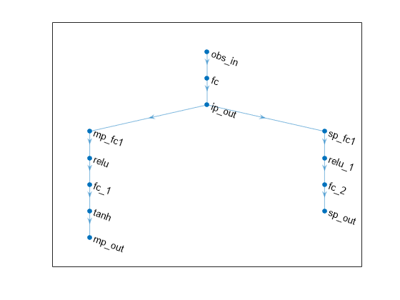
Define each network path as an array of layer objects, and assign names to the input and output layers of each path. These names allow you to connect the paths and then later explicitly associate the network input and output layers with the appropriate environment channel.

% Input path
inPath = [ 
    featureInputLayer(prod(obsInfo.Dimension),Name="obs_in")
    fullyConnectedLayer(32)   
    reluLayer(Name="ip_out") ];

% Mean path
meanPath = [
    fullyConnectedLayer(16,Name="mp_fc1")
    reluLayer
    fullyConnectedLayer(1)
    tanhLayer(Name="tanh"); % range: -1,1
    scalingLayer(Name="mp_out", ...
        Scale=actInfo.UpperLimit) % range: -2,2
        ]; 

% Standard deviation path
sdevPath = [
    fullyConnectedLayer(16,Name="sp_fc1")
    reluLayer            
    fullyConnectedLayer(1); 
    softplusLayer(Name="sp_out") % non negative
    ]; 

% Assemble dlnetwork object.
actorNet = dlnetwork;
actorNet = addLayers(actorNet,inPath);
actorNet = addLayers(actorNet,meanPath);
actorNet = addLayers(actorNet,sdevPath);

% Connect output of inPath to meanPath input.
actorNet = connectLayers(actorNet,"ip_out","mp_fc1/in");
% Connect output of inPath to variancePath input.
actorNet = connectLayers(actorNet,"ip_out","sp_fc1/in");

% Plot network.
plot(actorNet)

% Initialize network.
actorNet = initialize(actorNet);

% Display the number of weights.
summary(actorNet)

   Initialized: true

   Number of learnables: 1.1k

   Inputs:
      1   'obs_in'   2 features

Create the actor approximator object using actorNet, the environment specifications, and the names of the network input and output layers as input arguments. For more information, on continuous Gaussian actors, see rlContinuousGaussianActor.

actor = rlContinuousGaussianActor(actorNet, ...
    obsInfo,actInfo, ...
    ObservationInputNames="obs_in", ...
    ActionMeanOutputNames="mp_out", ...
    ActionStandardDeviationOutputNames="sp_out");

Check the actor with a random input observation.

getAction(actor,{rand(obsInfo.Dimension)})

ans = 1x1 cell array
    {[0.0963]}

Create the PG agent using the actor and the baseline critic.

agent = rlPGAgent(actor,baseline)

agent = 
  rlPGAgent with properties:

            AgentOptions: [1x1 rl.option.rlPGAgentOptions]
    UseExplorationPolicy: 1
         ObservationInfo: [1x1 rl.util.rlNumericSpec]
              ActionInfo: [1x1 rl.util.rlNumericSpec]
              SampleTime: 1

Specify options for the agent, including training options for the actor and critic.

agent.AgentOptions.UseBaseline = true;
agent.AgentOptions.DiscountFactor = 0.99;

agent.AgentOptions.CriticOptimizerOptions.LearnRate = 5e-3;
agent.AgentOptions.CriticOptimizerOptions.GradientThreshold = 1;

agent.AgentOptions.ActorOptimizerOptions.LearnRate = 5e-3;
agent.AgentOptions.ActorOptimizerOptions.GradientThreshold = 1;

Check your agent with a random input observation.

getAction(agent,{rand(obsInfo.Dimension)})

ans = 1x1 cell array
    {[1.1197]}

You can now test and train the agent within the environment.

Create a Discrete PG Agent with Recurrent Neural Networks

For this example, load the environment used in the example Train PG Agent with Custom Networks to Control Discrete Double Integrator. The observation from the environment is a vector containing the position and velocity of a mass. The action is a scalar representing a force, applied to the mass, having three possible values (-2, 0, or 2 Newton).

env = rlPredefinedEnv("DoubleIntegrator-Discrete");

Get observation and specification information.

obsInfo = getObservationInfo(env);
actInfo = getActionInfo(env);

Policy-gradient agents can optionally use a parametrized baseline function to approximate the value of the policy. To model the parametrized baseline function, use a recurrent neural network.

Define the network as an array of layer objects. To create a recurrent network, use a sequenceInputLayer as the input layer and include at least one lstmLayer.

baselineNet = [
    sequenceInputLayer(prod(obsInfo.Dimension))
    lstmLayer(32)
    reluLayer
    fullyConnectedLayer(1)
    ];

Convert to a dlnetwork object and display the number of weights.

baselineNet = dlnetwork(baselineNet);
summary(baselineNet)

   Initialized: true

   Number of learnables: 4.5k

   Inputs:
      1   'sequenceinput'   Sequence input with 2 dimensions

Create the baseline approximator object using baselineNet and the observation specification.

baseline = rlValueFunction(baselineNet,obsInfo);

Check the baseline critic with a random input observation.

getValue(baseline,{rand(obsInfo.Dimension)})

ans = single

-0.0065

Policy gradient agents use a parametrized stochastic policy, which for discrete action spaces is implemented by a discrete categorical actor.

A discrete categorical actor implements a parametrized stochastic policy for a discrete action space.

This actor takes an observation as input and returns as output a random action sampled (among the finite number of possible actions) from a categorical probability distribution.

Since the critic has a recurrent network, the actor must have a recurrent network too. The network must have with one input layer (which receives the content of the environment observation channel, as specified by obsInfo) and one output layer. The output layer must return a vector of probabilities for each possible action, as specified by actInfo.

Define the network as an array of layer objects.

actorNet = [
    sequenceInputLayer(prod(obsInfo.Dimension))
    lstmLayer(32)
    reluLayer
    fullyConnectedLayer(numel(actInfo.Elements))
    ];

Convert to a dlnetwork object and display the number of weights.

actorNet = dlnetwork(actorNet);
summary(actorNet)

   Initialized: true

   Number of learnables: 4.5k

   Inputs:
      1   'sequenceinput'   Sequence input with 2 dimensions

Create the actor using actorNet and the observation and action specifications.

actor = rlDiscreteCategoricalActor(actorNet,obsInfo,actInfo);

Check the actor with a random observation input.

getAction(actor,{rand(obsInfo.Dimension)})

ans = 1x1 cell array
    {[0]}

Create a PG agent using the actor and the baseline network.

agent = rlPGAgent(actor,baseline)

agent = 
  rlPGAgent with properties:

            AgentOptions: [1x1 rl.option.rlPGAgentOptions]
    UseExplorationPolicy: 1
         ObservationInfo: [1x1 rl.util.rlNumericSpec]
              ActionInfo: [1x1 rl.util.rlFiniteSetSpec]
              SampleTime: 1

Check the agent with a random observation input.

getAction(agent,{rand(obsInfo.Dimension)})

ans = 1x1 cell array
    {[0]}

To evaluate the agent using sequential observations, use the sequence length (time) dimension. For example, obtain actions for a sequence of 9 observations.

[action,state] = getAction(agent, ...
    {rand([obsInfo.Dimension 1 9])});

Display the action corresponding to the seventh element of the observation.

action = action{1};
action(1,1,1,7)

ans = 
0

You can now test and train the agent within the environment.

Tips

• For continuous action spaces, the rlPGAgent agent does not enforce the constraints set by the action specification, so you must enforce action space constraints within the environment.

Version History

Introduced in R2019a