Model Magnetic Levitation System Using NARX Network
This example creates a nonlinear autoregressive with exogenous inputs (NARX) model of a magnetic levitation system using the position (output) and voltage (input) measurements. The data was collected at a sampling interval of 0.01 seconds. For more information on estimating NARX networks using narxnet and nlarx, see Train NARX Networks Using idnlarx Instead of narxnet.
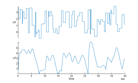
Prepare data for both the narxnet (Deep Learning Toolbox) and nlarx approaches.
[u,y] = maglev_dataset; % data represented by cell arrays (narxnet approach)
ud = cell2mat(u)';
yd = cell2mat(y)';
Ns = size(ud,1); % number of observations
time = seconds((0:Ns-1)*0.01)';
TT = timetable(time,ud,yd); % data represented by timetable (nlarx approach)
stackedplot(TT)
narxnet Approach
Create the series-parallel NARX network using narxnet (Deep Learning Toolbox). Use 10 neurons in the hidden layer and use the trainlm method (default) for training.
rng default
d1 = 1:2;
d2 = 1:2;
numUnits = 10;
model_narxnet = narxnet(d1,d2,numUnits);
model_narxnet.divideFcn = '';
model_narxnet.trainParam.min_grad = 1e-10;
model_narxnet.trainParam.showWindow = false;
[p,Pi,Ai,target] = preparets(model_narxnet,u,{},y);

model_narxnet = train(model_narxnet,p,target,Pi);
Simulate the network using the sim (Deep Learning Toolbox) command and convert the output to a numerical vector with initial conditions appended. Plot the resulting errors for the series-parallel implementation.
yp1 = sim(model_narxnet,p,Pi);
yp1 = [yd(1:2); cell2mat(yp1)'];
nlarx Approach
Create an idnlarx model that employs a one-hidden-layer network with 10 tanh units. Train the model using LM method, which is similar to the trainlm solver used by narxnet (Deep Learning Toolbox).
To use a neural network as a component of the nonlinear ARX model, use the idNeuralNetwork object. You can think of this object as a wrapper around a neural network which helps in its incorporation into the idnlarx model. idNeuralNetwork enables the use of networks from the Deep Learning Toolbox™ (dlnetwork (Deep Learning Toolbox)) and Statistics and Machine Learning Toolbox™ (RegressionNeuralNetwork (Statistics and Machine Learning Toolbox)) softwares.
rng default
UseLinear = false;
UseBias = false;

netfcn = idNeuralNetwork(10,"tanh",UseLinear,UseBias,NetworkType="dlnetwork");
OutputName = "yd";
InputName = "ud";
Reg = linearRegressor([OutputName, InputName],1:2);
model_nlarx = idnlarx(OutputName,InputName,Reg,netfcn);

opt = nlarxOptions(Focus="prediction",SearchMethod="lm");
opt.SearchOptions.MaxIterations = 15;
opt.SearchOptions.Tolerance = 1e-9;
opt.Display = "on";
opt.Normalize = false; % this is to match the default behavior of narxnet
model_nlarx = nlarx(TT,model_nlarx,opt)
model_nlarx =

Nonlinear ARX model with 1 output and 1 input
  Inputs: ud
  Outputs: yd

Regressors:
  Linear regressors in variables yd, ud
  List of all regressors

Output function: Deep learning network
Sample time: 0.01 seconds

Status:
Estimated using NLARX on time domain data "TT".
Fit to estimation data: 99.89% (prediction focus)
FPE: 2.491e-06, MSE: 2.415e-06

Model Properties
Predict one-step-ahead response using the predict command.
yp2 = predict(model_nlarx,TT,1);
Compare the generated responses using narxnet and nlarx approaches to the measured position data.
plot(time,yd,"k.",time,yp1,time,yp2.yd);
legend("measured","narxnet","nlarx")
title("One-step-ahead (open-loop) Prediction")
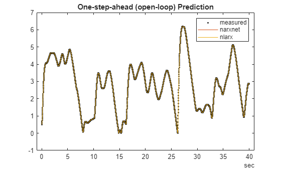
The plot indicates that both narxnet and nlarx methods predict the one-step-ahead response perfectly. Now assess their simulation (infinite-horizon prediction) abilities.
Prepare validation (test) data for both narxnet and nlarx approaches.
y1 = y(1700:2600);
yd1 = cell2mat(y1)';
u1 = u(1700:2600);
ud1 = cell2mat(u1)';
t = time(1700:2600);
Simulate the narxnet model in closed loop.
model_narxnetCL = closeloop(model_narxnet); % convert narxnet model into a recurrent model
[p1,Pi1,Ai1,t1] = preparets(model_narxnetCL,u1,{},y1);
ys1 = model_narxnetCL(p1,Pi1,Ai1);
ys1 = [yd1(1:2); cell2mat(ys1)'];
Simulate the nlarx model. You can do this using the sim command or predict command with a horizon of Inf. Here, you use predict.
ys2 = predict(model_nlarx,ud1,yd1,Inf);
Plot the simulated responses of the two models.
plot(t,yd1,t,ys1,t,ys2)
legend("measured","narxnet","nlarx")
title("Closed-loop Prediction (Simulation)")
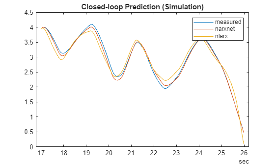
The simulation results match the measured data quite closely. You can retrieve the dlnetwork (Deep Learning Toolbox) embedded in the trained model.
fcn = model_nlarx.OutputFcn
fcn =
Multi-Layer Neural Network
Inputs: yd(t-1), yd(t-2), ud(t-1), ud(t-2)
Output: yd(t)

 Nonlinear Function: Deep learning network
         Contains 1 hidden layers using "tanh" activations.
         (uses Deep Learning Toolbox)
 Linear Function: not in use
 Output Offset: not in use

              Network: 'Deep learning network parameters'
            LinearFcn: 'Linear function parameters'
               Offset: 'Offset parameters'
    EstimationOptions: [1×1 struct]
net = fcn.Network
net =
Deep learning network parameters

    Parameters: 'Learnables and hyperparameters'
        Inputs: {'yd(t-1)'  'yd(t-2)'  'ud(t-1)'  'ud(t-2)'}
       Outputs: {'yd(t):Nonlinear'}
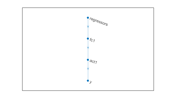
dlnet = getNetworkObj(net)
dlnet =
  dlnetwork with properties:

         Layers: [4×1 nnet.cnn.layer.Layer]
    Connections: [3×2 table]
     Learnables: [4×3 table]
          State: [0×3 table]
     InputNames: {'regressors'}
    OutputNames: {'y'}
    Initialized: 1

  View summary with summary.
plot(dlnet)
Other Configurations of Nonlinear ARX Models
The idnlarx models afford a significantly larger flexibility in choosing an appropriate structure for the dynamics. In addition to the multi-layer neural networks (created using the idNeuralNetwork object), there are several other choices, such as:
idWaveletNetwork— Wavelet networks for describing multi-scale dynamicsidTreeEnsemble,idTreePartition— Regression trees and forests of such trees (boosted, bagged)idGaussianProcess— Gaussian process regression mapsidSigmoidNetwork— Faster, one-hidden-layer neural networks usingsigmoidactivations
To use a neural network with a single hidden layer, using idSigmoidNetwork or idWaveletNetwork is more efficient than using idNeuralNetwork. For example, create a sigmoid network based nonlinear ARX model for the magnetic levitation system. Use 10 units of sigmoid activations in one hidden layer.
netfcn = idSigmoidNetwork(10); % 10 units of sigmoid activations in one hidden layerTrain the model for the default open-loop performance (Focus = "prediction").
model_sigmoidOL = nlarx(ud(1:2000),yd(1:2000),[2 2 1],netfcn)
model_sigmoidOL =

Nonlinear ARX model with 1 output and 1 input
  Inputs: u1
  Outputs: y1

Regressors:
  Linear regressors in variables y1, u1
  List of all regressors

Output function: Sigmoid network with 10 units
Sample time: 1 seconds

Status:
Estimated using NLARX on time domain data.
Fit to estimation data: 99.94% (prediction focus)
FPE: 8.477e-07, MSE: 7.935e-07

Model Properties
Train the model for closed-loop performance (Focus = "simulation").
opt = nlarxOptions(Focus="simulation");
opt.SearchMethod = "lm";
opt.SearchOptions.MaxIterations = 40;
model_sigmoidCL = nlarx(ud(1:2000),yd(1:2000),[2 2 1],netfcn,opt)
model_sigmoidCL =

Nonlinear ARX model with 1 output and 1 input
  Inputs: u1
  Outputs: y1

Regressors:
  Linear regressors in variables y1, u1
  List of all regressors

Output function: Sigmoid network with 10 units
Sample time: 1 seconds

Status:
Estimated using NLARX on time domain data.
Fit to estimation data: 94.41% (simulation focus)
FPE: 5.597e-07, MSE: 0.006894

Model Properties
Compare the closed-loop responses of the two models to measured test data. Rather than using the sim or predict commands, use the compare command. This command produces a plot overlaying the model results on the measured values and shows the percent fit to the data using the normalised root mean-squared error (NRMSE) measure (Fit = (1-NRMSE)*100).
close(gcf)
compare(ud(2001:end),yd(2001:end),model_sigmoidOL,model_sigmoidCL)
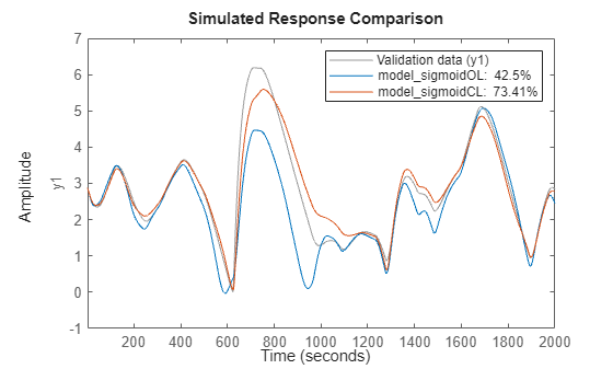
The plot shows the benefit of closed-loop training for predicting the response infinitely into the future.
See Also
train (Deep Learning Toolbox) | preparets (Deep Learning Toolbox) | closeloop (Deep Learning Toolbox) | narxnet (Deep Learning Toolbox) | idNeuralNetwork | idnlarx | nlarx | nlarxOptions | predict | iddata | linearRegressor | polynomialRegressor | getreg | periodicRegressor