Train NARX Networks Using idnlarx Instead of narxnet

Train NARX Networks Using `idnlarx` Instead of `narxnet`

This topic shows how to train a nonlinear autoregressive with exogenous inputs (NARX) network, that is, a nonlinear ARX model. You can use the idnlarx function from the System Identification Toolbox™ software instead of the narxnet (Deep Learning Toolbox) function from the Deep Learning Toolbox™ software.

About NARX Networks

A NARX network is a neural network that can learn to predict a time series given past values of the same time series, the feedback input, and possibly an auxiliary time series called the external (or exogenous) time series. The NARX network represents a prediction equation of the form

$y (t) = f (y (t - 1), y (t - 2), \dots, y (t - n a), u (t - 1), u (t - 2), \dots, u (t - n b)) .$

The value of the dependent output signal, y(t), is regressed on previous values of the output signal and previous values of an independent (exogenous) input signal, u(t). A finite number of lagged values of the output and inputs, if any, are denoted by na and nb in the equation, respectively. The values y(t) and u(t) can be multidimensional. This includes the situation where there are no exogenous inputs (that is, there is no available input u(t)). The corresponding model is a purely nonlinear autoregressive (NAR) model.

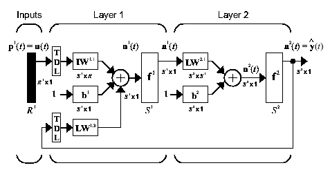
The function, $f (\cdot)$ , is represented by a multilayer feedforward neural network. For example, if the network has two layers, it takes this form:

A NARX network has many applications. You can use it to predict the next value of the signal. You can use it for nonlinear filtering, in which the target output is a noise-free version of the input signal. You can also use it in a black-box modeling approach to identify nonlinear dynamic systems.

In the Deep Learning Toolbox software, you can create a NARX network using the narxnet (Deep Learning Toolbox) command. The resulting network is represented by the network (Deep Learning Toolbox) object.

Alternatively, to create a NARX network, use the idnlarx model structure and the corresponding training command nlarx from the System Identification Toolbox software.

The advantages of using idnlarx instead of narxnet are:

You can specify different lag indices for different input and output variables when there are multiple inputs or outputs.
The idnlarx model structure allows the model regressors to be nonlinear functions of the lagged input/output variables.
You do not need to create separate open-loop and closed-loop variants of the trained model. You can use the same model for both the open-loop and closed-loop evaluations.
The idnlarx model structure offers specialized forms for certain single-hidden-layer networks. Using specialized forms can speed up the training.
You can use the idnlarx model structure to use the state-of-the-art numerical solvers from the Optimization Toolbox™ and Global Optimization Toolbox software. There are also several built-in line-search solvers available in the System Identification Toolbox software that are calibrated to handle small- to medium-scale problems efficiently.
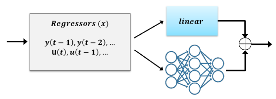
The idnlarx model structure allows physics-inspired learning. You can begin your modeling exercise with a simple linear model, which is derived by physical considerations or by using a linear model identification approach. You can then augment this linear model with a nonlinear function to improve its fidelity.
You can incorporate deep networks created using the Deep Learning Toolbox software and a variety of regression models from the Statistics and Machine Learning Toolbox™ software using the idNeuralNetwork object.
You can use an idnlarx model for N-step-ahead prediction, where N can vary from one to infinity. This type of prediction can be extremely useful for assessing the time horizon over which the model is usable.

Transition from `narxnet` to `idnlarx`

The narxnet (Deep Learning Toolbox) command originated in the historical shallow networks and employs terminology that is different from the current terminology used in the System Identification Toolbox software. This topic establishes the equivalence between the concepts and terminology used in both areas.

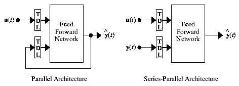
The narxnet and idnlarx model structures each represent two architectures: Parallel architecture (closed-loop) and Series-parallel architecture (open-loop).

You represent the parallel and series-parallel models using different network (Deep Learning Toolbox) objects in the Deep Learning Toolbox software. However, a single idnlarx model from the System Identification Toolbox software can serve both architectures. Depending on your application needs, you can run the idnlarx model in parallel (closed-loop) or series-parallel (open-loop) configurations.

Parallel Architecture

In the parallel case, the past output signal values used by the network (the terms y(t-1),y(t-2),... in the network equation) are estimated by the network itself at previous time steps. This is also called a recurrent or closed-loop model.

Closed-Loop narxnet Training and Simulation. Create an initial model using the narxnet (Deep Learning Toolbox) command. To create a parallel (closed-loop) configuration, specify feedbackMode to be "closed".

model = narxnet(inputDelays,feedbackDelays,hiddenSizes,"closed")
view(model)

The model, model, is a closed-loop network represented by the network (Deep Learning Toolbox) object. Train the parameters (weights and biases) of the model using the train (Deep Learning Toolbox) command.

model_closedloop = train(model,input_data,output_data,...)

You can compute the output of the trained model by using the sim (Deep Learning Toolbox) method of the network (Deep Learning Toolbox) object.

Closed-Loop idnlarx Training and Simulation. Create an initial model using the idnlarx command. You can do this without specifying the feedback mode. You specify the feedback mode during training as a value of the Focus training option.

net = idNeuralNetwork(LayerSizes)
model = idnlarx(output_name,input_name,[na nb nk],net)

Train the parameters (weights and biases) of the model using the nlarx command. Set the training option Focus to "simulation" using the nlarxOptions option set.

trainingOptions = nlarxOptions(Focus="simulation")
model = nlarx(data,model,trainingOptions)

In most situations, you can directly create the model by providing the orders and model structure information to the nlarx command, without first using idnlarx.

net = idNeuralNetwork(LayerSizes)
model = nlarx(data,[na nb nk],net,trainingOptions)

The model, model, is a nonlinear ARX model represented by the idnlarx object. You can compute the output of the trained model by using the sim method of the idnlarx object.

Series-Parallel Architecture

In the series-parallel case, the past output signal values used by the network (the terms y(t-1),y(t-2),... in the network equation) are provided externally as measured values of the output signals. This is also called a feedforward or open-loop model.

Open-Loop narxnet Training and Simulation. Create an initial model using the narxnet (Deep Learning Toolbox) command. To create a series-parallel (open-loop) configuration, specify feedbackMode to be "open" (default value).

model = narxnet(inputDelays,feedbackDelays,hiddenSizes)

model = narxnet(inputDelays,feedbackDelays,hiddenSizes,"open")
view(model)

The model, model, is an open-loop network represented by the network (Deep Learning Toolbox) object. Train the parameters (weights and biases) of the model using the train (Deep Learning Toolbox) command.

model_openloop = train(model,input_data,output_data,...)

You can compute the output of the trained model by using the sim (Deep Learning Toolbox) method of the network (Deep Learning Toolbox) object.

Open-Loop idnlarx Training and Simulation. Create an initial model using the idnlarx command. As in the closed-loop case, you can do this without specifying the feedback mode. You specify the feedback mode during training as a value of the Focus training option.

net = idNeuralNetwork(LayerSizes)
model = idnlarx(output_name,input_name,[na nb nk],net)

Train the parameters (weights and biases) of the model using the nlarx command. Set the training option Focus to "prediction" (default value) using the nlarxOptions option set.

trainingOptions = nlarxOptions(Focus="prediction")
model = nlarx(data,model,trainingOptions)

In most situations, you can directly train the model by providing the orders and model structure information to the nlarx command.

net = idNeuralNetwork(LayerSizes)
model = nlarx(data,[na nb nk],net,trainingOptions)

The model, model, is a nonlinear ARX model represented by the idnlarx object. Structurally, it is the same as the closed-loop model. So, you require different commands to compute the open-loop and closed-loop simulation results. You compute the closed-loop simulation results using the sim command. For open-loop results, use the predict command with a prediction horizon of one.

y = predict(model,past_data,1)   % open-loop simulation

You can also use the predict command for obtaining the closed-loop simulation results by using a prediction horizon of Inf.

y = predict(model,past_data,Inf) % closed-loop simulation

When using narxnet, the closed-loop model (parallel) is structurally different from the open-loop model (series-parallel). To use an open-loop network for closed-loop simulations, you need to explicitly convert the open-loop network into a closed-loop network. To do this, use the closeloop (Deep Learning Toolbox) command.

[model_closedloop,Xic,Aic] = closeloop(model_openloop,Xf,Af);

When using nlarx, you do not need any conversion since the open-loop trained model is structurally identical to the closed-loop trained model. Instead, you choose between the sim and predict commands, as shown above.

Data Format

This example uses:

Open Live Script

narxnet (Deep Learning Toolbox) training requires the input and output time series (signals) to be provided as cell arrays. Each element of the cell array represents one observation at a given time instant. For multivariate signals, each cell element must contain as many rows as there are variables. Suppose the training data for a process with one output and two inputs is:

Time (t)	Input 1 (u1)	Input 2 (u2)	Output (y)
0	1	5	100
0.1	2	-2	500
0.2	0	4	-100
0.3	10	34	-200

The format of the input data for training must be:

% input data
u = {[1; 5], [2; -2], [0; 4], [10; 34]};
% output data
y = {100, 500, -100, -200};

Furthermore, before using the data for training, you must shift it according to different lag values (na and nb) explicitly. Create the NARX network using narxnet (Deep Learning Toolbox) and prepare time series data using the preparets (Deep Learning Toolbox) command.

na = 2; % y(t-1), y(t-2)
nb = 3; % u1(t-1), u1(t-2), u1(t-3), u2(t-1), u2(t-2), u3(t-3) 
net = narxnet(1:nb,1:na,10);
[u_shifted,u_delay_states,layer_delay_states,y_shifted] = preparets(net,u,{},y)

u_shifted=2×1 cell array
    {2×1 double}
    {[    -200]}

u_delay_states=2×3 cell array
    {2×1 double}    {2×1 double}    {2×1 double}
    {[     100]}    {[     500]}    {[    -100]}

layer_delay_states =

  2×0 empty cell array

y_shifted = 1×1 cell array
    {[-200]}

Train the model.

% net = train(net,u_shifted,y_shifted,u_delay_states,layer_delay_states);

In contrast, nlarx requires the data to be specified as double matrices with variables along the columns and the observations along the rows. You can use a pair of double matrices to specify the data.

% input data
u1 = [1 2 0 10]';
u2 = [5 -2 4 34]';
u = [u1, u2];
% output data
y = [100, 500, -100, -200]';

Train the model.

% model = nlarx(u,y,[na nb nk],network_structure)

Alternatively, use a timetable for the data (recommended syntax). The benefit of using a timetable is that the knowledge of the time vector is retained and carried over to the model. You can also specify the names of the input variables, if needed.

target = seconds(0:0.1:0.3)';
tt = timetable(target,u1,u2,y)

tt=4×3 timetable
    target     u1    u2     y  
    _______    __    __    ____

    0 sec       1     5     100
    0.1 sec     2    -2     500
    0.2 sec     0     4    -100
    0.3 sec    10    34    -200

Train the model.

% model = nlarx(tt,[na nb nk],network_structure)

Similarly, you can replace a timetable with an iddata object.

dat = iddata(y,u,0.1,Tstart=0);

Train the model.

% model = nlarx(dat,[na nb nk],network_structure)

Model Order Specification

The narxnet (Deep Learning Toolbox) function requires you to specify the lags to use for the input and output variables. In the multi-output case (that is, the number of output variables > 1), the lags used for all output variables must match. Similarly, the lags used for all input variables must match.

input_lags = 0:3;
output_lags = 1:2;
hiddenLayerSizes = [10 5]; % two hidden layers
model = narxnet(input_lags,output_lags,hiddenLayerSizes);

You use the specified lags to generate the input features or predictors, also called regressors. For the above example, these regressors are: $y (t - 1)$ , $y (t - 2)$ , $u_{1} (t)$ , $u_{1} (t - 1)$ , $u_{1} (t - 2)$ , $u_{1} (t - 3)$ , $u_{2} (t)$ , $u_{2} (t - 1)$ , $u_{2} (t - 2)$ , and $u_{2} (t - 3)$ , where $y (t)$ denotes the output signal, and $u_{1} (t), u_{2} (t)$ denote the two input signals. In the system identification terminology, these are called linear regressors.

When using the idnlarx framework, you create the linear, consecutive-lag regressors by specifying the maximum lag in each output (na), the minimum lags in the two inputs (nk), and the total number of input variable lags (nb). You put these numbers together in a single order matrix. You can pick different lags for different input and output variables.

na = 2;     % maximum output lag
nb = [4 2]; % total number of consecutive lags in the two inputs
nk = [0 5]; % minimum lags in the two inputs
hiddenLayerSizes = [10 5]; % two hidden layers
netfcn = idNeuralNetwork(hiddenLayerSizes,NetworkType="dlnetwork");
model = idnlarx("y",["u1", "u2"],[na nb nk],netfcn)

model =

Nonlinear ARX model with 1 output and 2 inputs
  Inputs: u1, u2
  Outputs: y

Regressors:
  Linear regressors in variables y, u1, u2
  List of all regressors

Output function: Deep learning network
Sample time: 1 seconds

Status:                                                         
Created by direct construction or transformation. Not estimated.

Model Properties

You can generate the formulas of the regressors resulting from the above lags programmatically using getreg.

getreg(model)

ans = 8×1 cell
    {'y(t-1)' }
    {'y(t-2)' }
    {'u1(t)'  }
    {'u1(t-1)'}
    {'u1(t-2)'}
    {'u1(t-3)'}
    {'u2(t-5)'}
    {'u2(t-6)'}

With idnlarx models, you can incorporate more complex forms of regressors, such as $| y (t - 1) |$ , $y (t - 2) u (t - 5)$ , $u^{3} (t)$ , $s i n (2 π \cdot u (t - 1))$ , and so on. To do this, use the dedicated regressor creator functions: linearRegressor, polynomialRegressor, periodicRegressor, and customRegressor. Some examples are:

vars = ["y","u1","u2"];
% Absolute valued regressors for "y" and "u1"
UseAbs = true; 
R1 = linearRegressor(vars(1:2),1:2,UseAbs)

R1 = 
Linear regressors in variables y, u1
       Variables: {'y'  'u1'}
            Lags: {[1 2]  [1 2]}
     UseAbsolute: [1 1]
    TimeVariable: 't'

  Regressors described by this set

getreg(R1)

ans = 4×1 string
    "|y(t-1)|"
    "|y(t-2)|"
    "|u1(t-1)|"
    "|u1(t-2)|"

% Second order polynomial regressors with different lags for each variable
UseAbs = false;
UseLagMix = true;
R2 = polynomialRegressor(vars,{[1 2],0,[4 9]},2,UseAbs,false,UseLagMix)

R2 = 
Order 2 regressors in variables y, u1, u2
               Order: 2
           Variables: {'y'  'u1'  'u2'}
                Lags: {[1 2]  [0]  [4 9]}
         UseAbsolute: [0 0 0]
    AllowVariableMix: 0
         AllowLagMix: 1
        TimeVariable: 't'

  Regressors described by this set

getreg(R2)

ans = 7×1 string
    "y(t-1)^2"
    "y(t-2)^2"
    "y(t-1)*y(t-2)"
    "u1(t)^2"
    "u2(t-4)^2"
    "u2(t-9)^2"
    "u2(t-4)*u2(t-9)"

% Periodic regressors in "u2" with lags 0, 4
% Generate three Fourier terms with a fundamental frequency of pi. Generate both sine and cosine functions.
R3 = periodicRegressor(vars(3),[0 4],pi,3)

R3 = 
Periodic regressors in variables u2 with 3 Fourier terms
       Variables: {'u2'}
            Lags: {[0 4]}
               W: 3.1416
        NumTerms: 3
          UseSin: 1
          UseCos: 1
    TimeVariable: 't'
     UseAbsolute: 0

  Regressors described by this set

getreg(R3)

ans = 12×1 string
    "sin(3.142*u2(t))"
    "sin(2*3.142*u2(t))"
    "sin(3*3.142*u2(t))"
    "cos(3.142*u2(t))"
    "cos(2*3.142*u2(t))"
    "cos(3*3.142*u2(t))"
    "sin(3.142*u2(t-4))"
    "sin(2*3.142*u2(t-4))"
    "sin(3*3.142*u2(t-4))"
    "cos(3.142*u2(t-4))"
    "cos(2*3.142*u2(t-4))"
    "cos(3*3.142*u2(t-4))"

You can replace the orders matrix with a vector of regressors in the idnlarx or the nlarx command.

regressors = [R1 R2 R3];
model = idnlarx("y",["u1", "u2"],regressors,netfcn);
getreg(model)

ans = 23×1 cell
    {'|y(t-1)|'            }
    {'|y(t-2)|'            }
    {'|u1(t-1)|'           }
    {'|u1(t-2)|'           }
    {'y(t-1)^2'            }
    {'y(t-2)^2'            }
    {'y(t-1)*y(t-2)'       }
    {'u1(t)^2'             }
    {'u2(t-4)^2'           }
    {'u2(t-9)^2'           }
    {'u2(t-4)*u2(t-9)'     }
    {'sin(3.142*u2(t))'    }
    {'sin(2*3.142*u2(t))'  }
    {'sin(3*3.142*u2(t))'  }
    {'cos(3.142*u2(t))'    }
    {'cos(2*3.142*u2(t))'  }
    {'cos(3*3.142*u2(t))'  }
    {'sin(3.142*u2(t-4))'  }
    {'sin(2*3.142*u2(t-4))'}
    {'sin(3*3.142*u2(t-4))'}
    {'cos(3.142*u2(t-4))'  }
    {'cos(2*3.142*u2(t-4))'}
    {'cos(3*3.142*u2(t-4))'}

Network Structure Specification

The narxnet (Deep Learning Toolbox) command does not allow you to pick the types of activation functions used by each hidden layer. It uses the tanh activation function in all the layers. In contrast, you can create idnlarx networks that use a variety of different activation functions. You can also use custom networks, which are, for example, created using the Deep Network Designer app.

Examples

For examples on creating a NARX network using both narxnet and nlarx functions, see Train and Simulate Simple NARX Network and Model Magnetic Levitation System Using NARX Network.