compreal

Compute companion state-space realization

Since R2023b

Syntax

csys = compreal(sys)

csys = compreal(sys,type)

[csys,T] = compreal(___)

Description

csys = compreal(sys) returns the controllable companion realization of the single-input LTI model sys.

csys = compreal(sys,type) returns the realization of the model sys depending on type. Specify type as "c" for controllable companion form or "o" for observable companion form.

• "c" — Computes the controllable companion realization for a single-input LTI model sys. This is the same as the first syntax.

• "o" — Computes the observable companion realization for a single-output LTI model sys.

[csys,T] = compreal(___) also returns the transformation matrix T for explicit models with matrices A, B, C such that

• The controllable companion form is T^-1AT, T^-1B, CT.

• The observable companion form is TAT^-1, TB, CT^-1.

Examples

Convert State-Space Model to Companion Canonical Form

aircraftPitchSSModel.mat contains the state-space matrices of an aircraft where the input is elevator deflection angle $\delta$ and the output is the aircraft pitch angle $\theta$.

$$\begin{array}{l}\left[\begin{array}{c}\underset{}{\overset{\dot{}}{\alpha }}\\ \underset{}{\overset{\dot{}}{q}}\\ \underset{}{\overset{\dot{}}{\theta }}\end{array}\right]=\left[\begin{array}{ccc}-0.313& 56.7& 0\\ -0.0139& -0.426& 0\\ 0& 56.7& 0\end{array}\right]\left[\begin{array}{c}\alpha \\ q\\ \theta \end{array}\right]+\left[\begin{array}{c}0.232\\ 0.0203\\ 0\end{array}\right]\left[\delta \right]\\ y=\left[\begin{array}{ccc}0& 0& 1\end{array}\right]\left[\begin{array}{c}\alpha \\ q\\ \theta \end{array}\right]+\left[0\right]\left[\delta \right]\end{array}$$

Load the model data to the workspace and create the state-space model sys.

load('aircraftPitchSSModel.mat');
sys = ss(A,B,C,D)

sys =
 
  A = 
            x1       x2       x3
   x1   -0.313     56.7        0
   x2  -0.0139   -0.426        0
   x3        0     56.7        0
 
  B = 
           u1
   x1   0.232
   x2  0.0203
   x3       0
 
  C = 
       x1  x2  x3
   y1   0   0   1
 
  D = 
       u1
   y1   0
 
Continuous-time state-space model.

Convert the resultant state-space model sys to controllable companion form.

csys = compreal(sys)

csys =
 
  A = 
              x1         x2         x3
   x1          0          0  1.914e-15
   x2          1          0    -0.9215
   x3          0          1     -0.739
 
  B = 
       u1
   x1   1
   x2   0
   x3   0
 
  C = 
            x1       x2       x3
   y1        0    1.151  -0.6732
 
  D = 
       u1
   y1   0
 
Continuous-time state-space model.

csys is the controllable companion form of sys.

Convert System to Observable Companion Form

The file icEngine.mat contains one data set with 1500 input-output samples collected at a sampling rate of 0.04 seconds. The input u(t) is the voltage (V) controlling the By-Pass Idle Air Valve (BPAV), and the output y(t) is the engine speed (RPM/100).

Use the data in icEngine.mat to create a state-space model with identifiable parameters.

load icEngine.mat
z = iddata(y,u,0.04);
sys = n4sid(z,4,'InputDelay',2);

Convert the identified state-space model sys to observable companion form.

[osys,T] = compreal(sys,"o");

Compare frequency response confidence bounds of sys to osys.

h = bodeplot(sys,osys,'r.');
showConfidence(h)

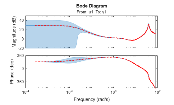
The frequency response confidence bounds are identical.

Additionally, compreal returns a transformation matrix T such that the observable companion form is ${\mathit{A}}_{\mathit{o}}={\mathit{TAT}}^{-1}$, ${\mathit{B}}_{\mathit{o}}=\mathit{TB}$, ${\mathit{C}}_{\mathit{o}}={\mathit{CT}}^{-1}$.

Input Arguments

sys — Dynamic system

dynamic system model

Dynamic system, specified as a SISO, or MIMO dynamic system model. Dynamic systems that you can use include:

• Continuous-time or discrete-time numeric LTI models, such as tf (Control System Toolbox), zpk (Control System Toolbox), ss (Control System Toolbox), or pid (Control System Toolbox) models.

• Generalized or uncertain LTI models such as genss (Control System Toolbox) or uss (Robust Control Toolbox) models. (Using uncertain models requires Robust Control Toolbox™ software.)

• Identified LTI models, such as idtf, idss, idproc, idpoly, and idgrey models.

You cannot use frequency-response data models such as frd (Control System Toolbox) models.

type — Companion realization type

"c" (default) | "o"

Companion realization type, specified as "c" (controllable companion form) or "o" (observable companion form).

For a system with characteristic polynomial

$$P(s)=s^n+{\alpha }_{n-1}{s}^{n-1}+{\alpha }_{n-2}{s}^{n-2}+\dots +{\alpha }_{1}s+{\alpha }_0,$$

the function returns the companion forms as follows.

• Controllable Companion Form

  In the controllable companion realization, the characteristic polynomial of the system appears explicitly in the rightmost column of the A matrix.

  $$A_{ccom}=\left[\begin{array}{ccc}\begin{array}{l}0\\ 1\\ 0\\ 0\\ ⋮\\ 0\end{array}& \begin{array}{l}0\\ 0\\ 1\\ 0\\ ⋮\\ 0\end{array}& \begin{array}{ccc}\begin{array}{cc}\begin{array}{l}0\\ 0\\ 0\\ 1\\ ⋮\\ 0\end{array}& \begin{array}{l}\dots \\ \dots \\ \dots \\ \dots \\ \ddots \\ \dots \end{array}\end{array}& \begin{array}{l}0\\ 0\\ 0\\ 0\\ ⋮\\ 1\end{array}& \begin{array}{l}-{\alpha }_0\\ -{\alpha }_1\\ -{\alpha }_2\\ -{\alpha }_3\\ ⋮\\ -{\alpha }_{n-1}\end{array}\end{array}\end{array}\right],B_{ccom}=\left[\begin{array}{c}1\\ 0\\ ⋮\\ 0\end{array}\right].$$

• Observable Companion Form

  In the observable companion realization, the characteristic polynomial of the system appears explicitly in the last row of the A matrix.

  $$A_{ocom}=\left[\begin{array}{ccc}\begin{array}{l}0\\ 0\\ 0\\ ⋮\\ 0\\ -{\alpha }_0\end{array}& \begin{array}{l}1\\ 0\\ 0\\ ⋮\\ 0\\ -{\alpha }_1\end{array}& \begin{array}{ccc}\begin{array}{cc}\begin{array}{l}0\\ 1\\ 0\\ ⋮\\ 0\\ -{\alpha }_2\end{array}& \begin{array}{l}0\\ 0\\ 1\\ ⋮\\ 0\\ -{\alpha }_3\end{array}\end{array}& \begin{array}{l}\dots \\ \dots \\ \dots \\ \ddots \\ \dots \\ \dots \end{array}& \begin{array}{l}0\\ 0\\ 0\\ ⋮\\ 1\\ -{\alpha }_{n-1}\end{array}\end{array}\end{array}\right],C_{ocom}=\left[\begin{array}{cccc}1& 0& \dots & 0\end{array}\right].$$

For more information, see State-Space Realizations.

Output Arguments

csys — Companion state-space form of the dynamic model

ss model object

Companion state-space form of the dynamic model, returned as an ss (Control System Toolbox) model object. csys is a state-space realization of sys in the companion form specified by type (controllable or observable).

T — Transformation matrix

matrix | []

Transformation matrix, returned as an n-by-n matrix, where n is the number of states.

• For explicit state-space models with matrices A, B, C, the function returns T such that

  • The controllable companion form is T^-1AT, T^-1B, CT.

  • The observable companion form is TAT^-1, TB, CT^-1.

• For descriptor state-space models, the function always returns an empty value [].

Tips

Computing companion realizations often involves ill-conditioned transformations and loss of accuracy. Use modalreal or balreal as numerically stable alternatives.

Version History

Introduced in R2023b