Hydromechanical 4-Way Directional Valve with Force Actuation

R2026b

Since R2026b

This example shows how to build a 4-way directional valve using components from the Hydromechanical Valves library. The valve experiences mechanical effects such as mass and damping on the dynamic response of the valve spool.

model = "Hydromechanical4WayDirectionalValve";
open_system(model)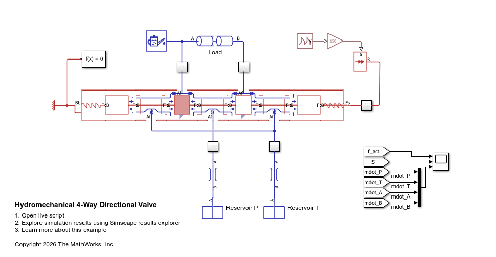

Model Overview

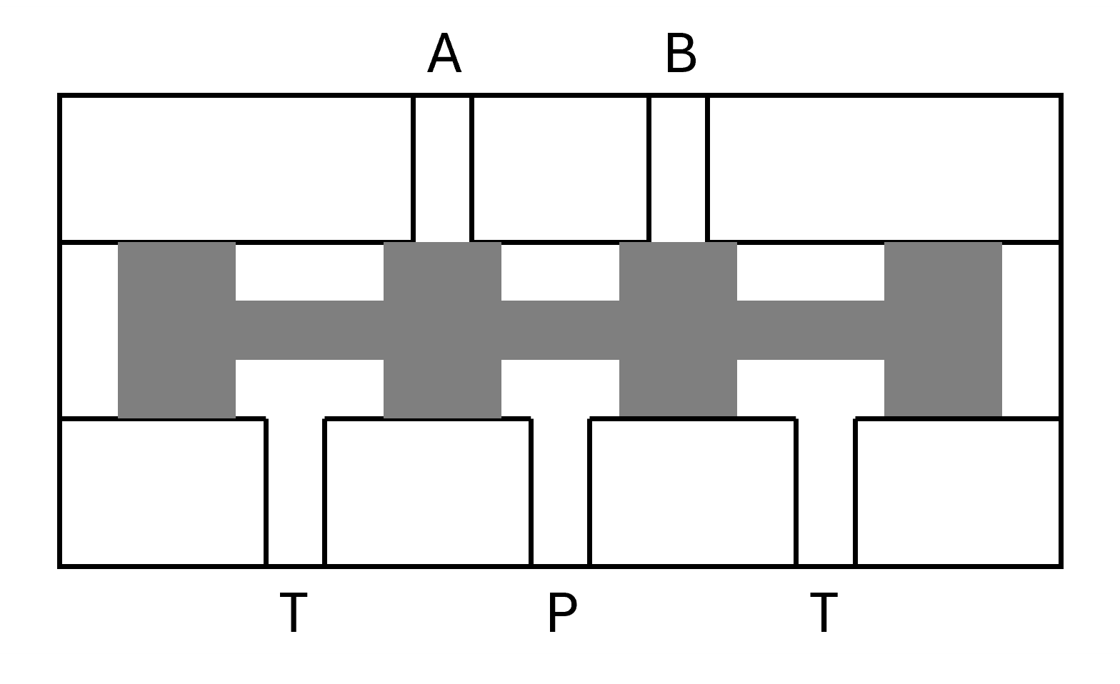
The following diagram illustrates a 4-way directional valve with its spool in the neutral position. It is an overlapped spool valve where the lands are wider than the ports. Therefore, the fluid is blocked in the neutral position. There are four fluid ports: P, T, A, and B. The two T ports shown in the diagram are assumed to be connected by a fluid channel in the valve body so they act as a single port.

When the spool moves to the left, it creates fluid flow paths between ports P and A and between ports B and T.

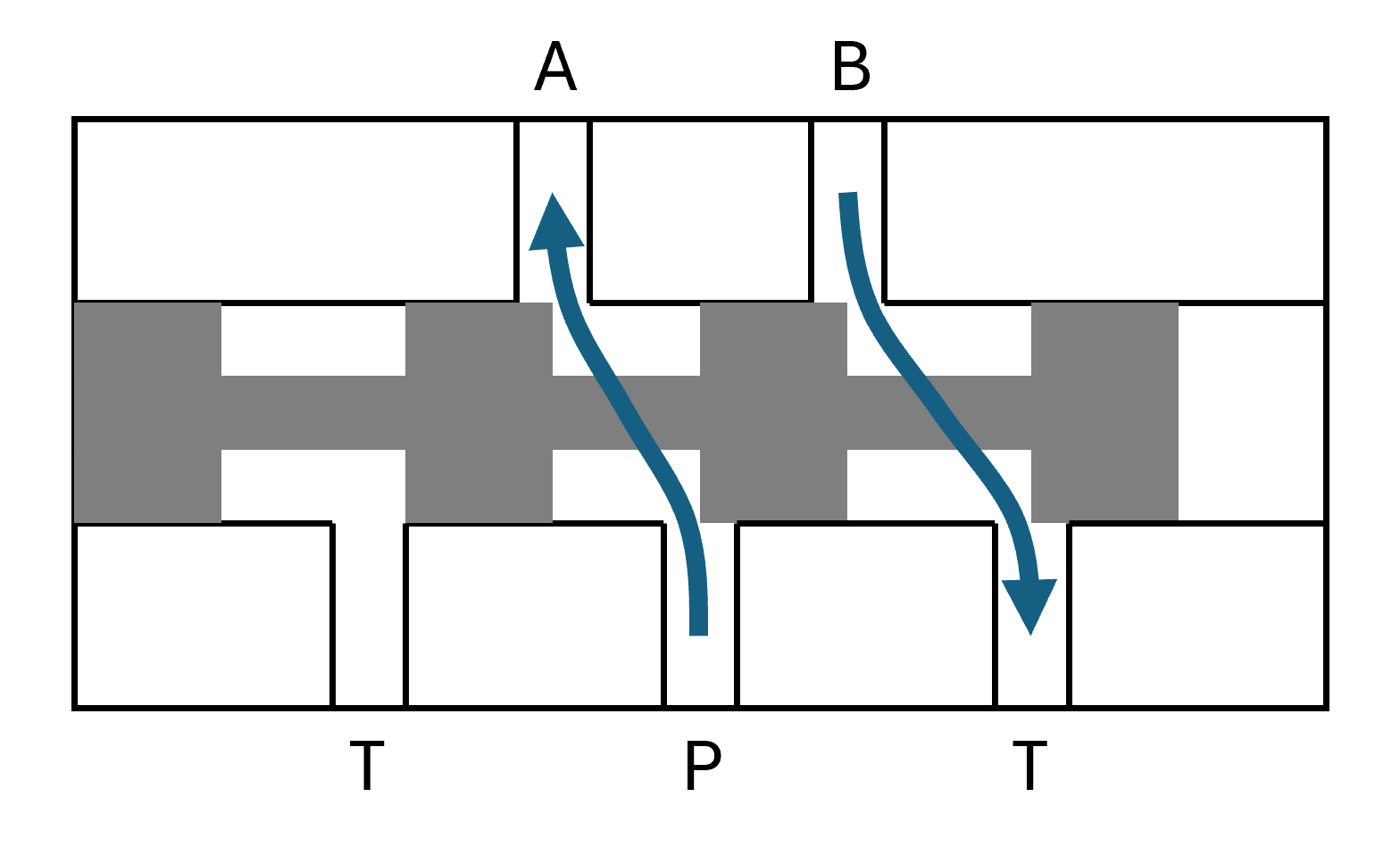
When the spool moves to the right, it creates fluid flow paths between ports P and B and between ports A and T.

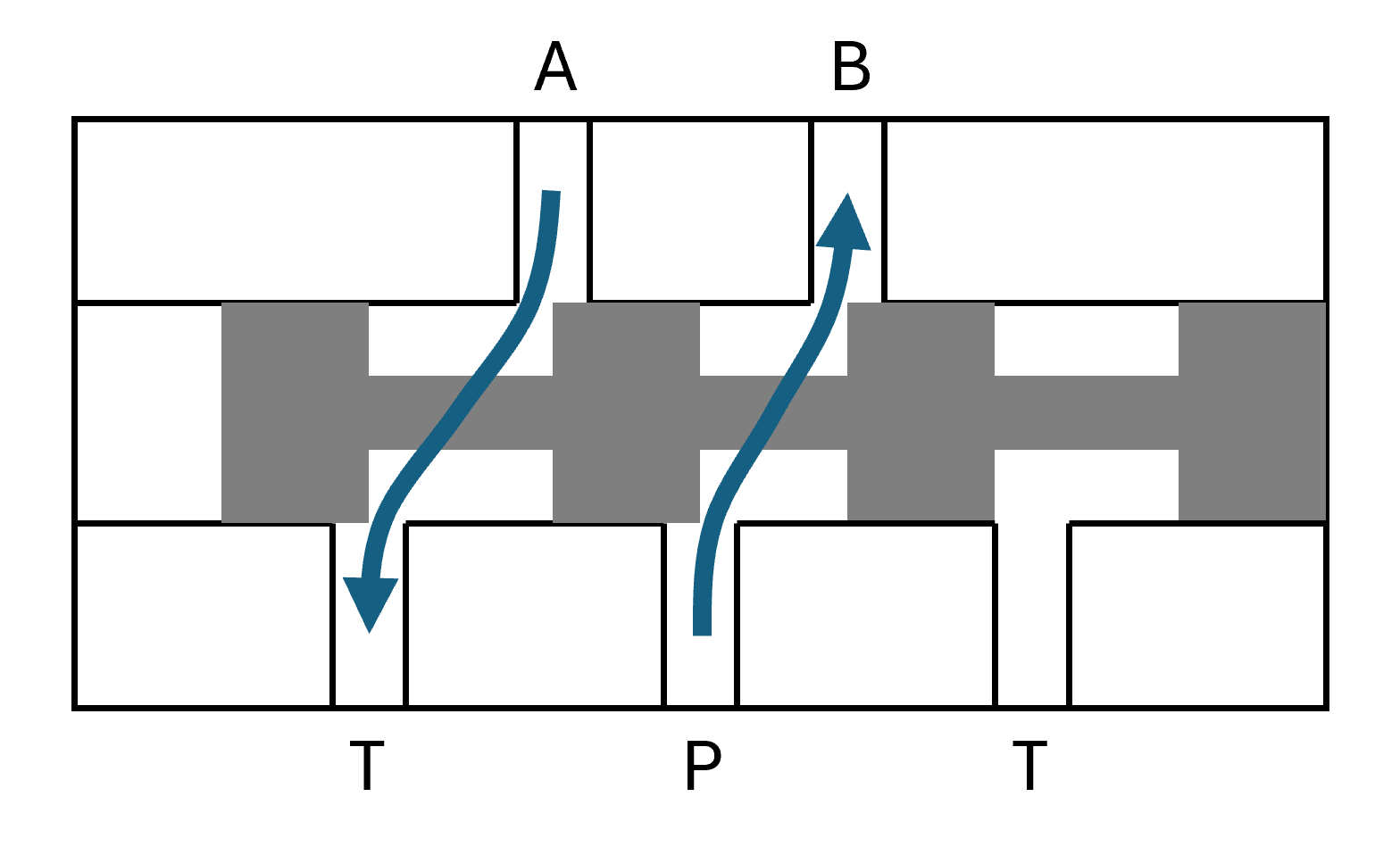
Each block in the Hydromechanical Valves library models a piece of a valve that you combine to model a complete valve. The block icons are intended to be arranged next to each other to resemble a valve schematic, but they must still be connected together via their B and F hydromechanical valve ports. The figure below shows the model with the individual blocks identified and spaced apart to show the connection lines.

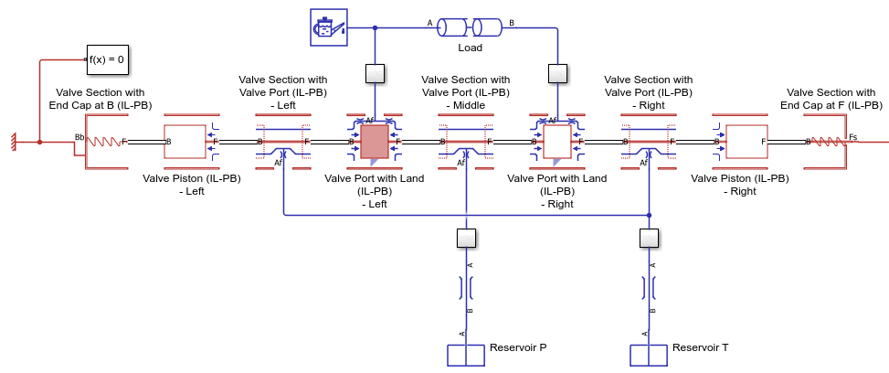
The 4-way directional valve model consists of the following hydromechanical valve blocks:

Valve Section with End Cap at B (IL-PB) - models the terminal section on the left side of the valve and defines the reference position for the entire valve structure.
Valve Section with End Cap at F (IL-PB) - models the terminal section on the right side of the valve and provides a connection point for the valve actuator that moves the spool.
Valve Port with Land (IL-PB) - models the two valve ports, A and B, and the two spool lands that meter flow through those ports.
Valve Section with Valve Port (IL-PB) - models the three sections with spool shafts that rigidly connect the lands in adjacent blocks as well as the valve ports P and T which are metered by those lands.
Valve Piston (IL-PB) - models the two spool lands next to the end caps that keep the fluid contained within the spool.

For more information, see Get Started with the Hydromechanical Valve Library.

Model Setup

The model Hydromechanical4WayDirectionalValve is already fully configured and ready to simulate a 4-way directional valve. This section highlights the key steps in configuring the model.

Although the Valve Section with Valve Port (IL-PB) blocks do not model the lands themselves, they still model the flow metering caused by the adjacent lands moving over their valve ports. Thus, Valve Section with Valve Port (IL-PB) blocks should always be adjacent to blocks that model the lands. In this model, the lands modeled by the Valve Port with Land (IL-PB) blocks can each meter three valve ports: the port in the Valve Port with Land (IL-PB) block itself, the port in the Valve Section with Valve Port (IL-PB) block to its left, and the port in the Valve Section with Valve Port (IL-PB) block to its right.

Ports Af in the leftmost and the rightmost Valve Section with Valve Port (IL-PB) blocks are connected because the fluid goes to a single valve port T. You may replace this direct connection with a block such as a Pipe (IL) block or a Flow Resistance (IL) block to model additional effects.

The leftmost and rightmost spool lands block fluid flow inside the valve. Therefore, the two end cap valve sections do not contain fluid. First, configure the Valve Piston (IL-PB) blocks such that the side next to the end cap valve sections do not contain fluid:

set_param(model + "/Valve Piston (IL-PB) - Left", "contains_liquid_B", "false")
set_param(model + "/Valve Piston (IL-PB) - Right", "contains_liquid_F", "false")

Next, configure the two end cap valve sections. When a valve section is configured to contain no fluid, the block assumes it is open to the atmosphere.

set_param(model + "/Valve Section with End Cap at B (IL-PB)", "contains_liquid", "false")
set_param(model + "/Valve Section with End Cap at F (IL-PB)", "contains_liquid", "false")

Note that if you do not set contains_liquid to false in the two end cap valve sections, the icons will show the blue isothermal liquid lines to indicate that there is fluid inside. The blue lines will not match up with any blue lines in the adjacent block icons. This mismatch in adjacent icons is a visual indication that the model is not configured correctly.

All mechanical models, including hydromechanical valve models, need a reference point to define the zero position. In this model, the left end cap is the reference position. Therefore, expose the position-based translational port Bb for the valve body and connect it to the Translational World (PB) block.

set_param(model + "/Valve Section with End Cap at B (IL-PB)", "enable_cap_port", "true")

In order to move the spool, you need a connection point to connect an actuator. Expose a position-based translational port Fs for the spool on the right end cap and connect it to an External Force Source (PB) block.

set_param(model + "/Valve Section with End Cap at B (IL-PB)", "enable_shaft_port", "true")

Valve port P is the pressure port, so it is connected to a reservoir at 0.201325 MPa. Valve port T is the tank port, so it is connected to a reservoir at 0.101325 MPa. Valve ports A and B are the working ports connected to a load. A Pipe (IL) block configured to have a large pressure drop models the load abstractly.

Model Parameters

After configuring the model, parameterize the blocks to define the spacing between the valve ports along the valve body and between the lands along the spool. When referring to the geometry, the "valve axial direction" refers to the translational motion direction of the moving valve element, which is the spool in this model. The "radial direction" and the "circumferential direction" are then defined assuming that the valve is axisymmetric.

Model all valve ports as simple rectangular slots with the same width along the valve axis and length along the circumference:

W_port = 0.02; % m
L_port = 0.1; % m
set_param(model + "/Valve Port with Land (IL-PB) - Left", "port_width", "W_port")
set_param(model + "/Valve Port with Land (IL-PB) - Left", "port_length", "L_port")
set_param(model + "/Valve Port with Land (IL-PB) - Right", "port_width", "W_port")
set_param(model + "/Valve Port with Land (IL-PB) - Right", "port_length", "L_port")
set_param(model + "/Valve Section with Valve Port (IL-PB) - Left", "port_width", "W_port")
set_param(model + "/Valve Section with Valve Port (IL-PB) - Left", "port_length", "L_port")
set_param(model + "/Valve Section with Valve Port (IL-PB) - Middle", "port_width", "W_port")
set_param(model + "/Valve Section with Valve Port (IL-PB) - Middle", "port_length", "L_port")
set_param(model + "/Valve Section with Valve Port (IL-PB) - Right", "port_width", "W_port")
set_param(model + "/Valve Section with Valve Port (IL-PB) - Right", "port_length", "L_port")

The spool land width along the valve axis for all four lands is

W_land = 0.1; % m
set_param(model + "/Valve Port with Land (IL-PB) - Left", "land_width", "W_land")
set_param(model + "/Valve Port with Land (IL-PB) - Right", "land_width", "W_land")
set_param(model + "/Valve Piston (IL-PB) - Left", "piston_width", "W_land")
set_param(model + "/Valve Piston (IL-PB) - Right", "piston_width", "W_land")

The fluid inside the valve occupies the annular area around the spool. Therefore, the annular area of the land will experience pressure force from the liquid.

D_land_outer = 0.1; % m
D_land_inner = 0.05; % m
A_land = pi*(D_land_outer^2 - D_land_inner^2)/4

A_land = 
0.0059

set_param(model + "/Valve Port with Land (IL-PB) - Left", "land_area_B", "pi*(D_land_outer^2 - D_land_inner^2)/4")
set_param(model + "/Valve Port with Land (IL-PB) - Left", "land_area_F", "pi*(D_land_outer^2 - D_land_inner^2)/4")
set_param(model + "/Valve Port with Land (IL-PB) - Right", "land_area_B", "pi*(D_land_outer^2 - D_land_inner^2)/4")
set_param(model + "/Valve Port with Land (IL-PB) - Right", "land_area_F", "pi*(D_land_outer^2 - D_land_inner^2)/4")
set_param(model + "/Valve Piston (IL-PB) - Left", "piston_area_F", "pi*(D_land_outer^2 - D_land_inner^2)/4")
set_param(model + "/Valve Piston (IL-PB) - Right", "piston_area_B", "pi*(D_land_outer^2 - D_land_inner^2)/4")

The valve section blocks define the spacing along the valve body between the center of the valve ports. Assume equal distance between the valve ports:

L_body = 0.1; % m
set_param(model + "/Valve Section with Valve Port (IL-PB) - Left", "body_length_F", "L_body")
set_param(model + "/Valve Section with Valve Port (IL-PB) - Middle", "body_length_B", "L_body")
set_param(model + "/Valve Section with Valve Port (IL-PB) - Middle", "body_length_F", "L_body")
set_param(model + "/Valve Section with Valve Port (IL-PB) - Right", "body_length_B", "L_body")

The distances between the two end caps and the leftmost and rightmost valve ports are longer to account for the width of the leftmost and rightmost lands. The reason for this is because the Valve Piston (IL-PB) block does not model valve body length.

set_param(model + "/Valve Section with End Cap at B (IL-PB)", "body_length", "L_body + W_land")
set_param(model + "/Valve Section with End Cap at F (IL-PB)", "body_length", "L_body + W_land")

The valve section blocks also define the spacing along the spool shaft between the lands. Assume equal distance between the spool lands:

L_shaft = 0.1; % m
set_param(model + "/Valve Section with Valve Port (IL-PB) - Left", "shaft_length", "L_shaft")
set_param(model + "/Valve Section with Valve Port (IL-PB) - Middle", "shaft_length", "L_shaft")
set_param(model + "/Valve Section with Valve Port (IL-PB) - Right", "shaft_length", "L_shaft")

An extra shaft is connected to the rightmost spool land and extends out beyond the right end cap. The actuator is attached to the end of this extra shaft.

L_shaft_end = 0.2; % m
set_param(model + "/Valve Section with End Cap at F (IL-PB)", "shaft_length", "L_shaft_end")

Finally, specify the area of the fluid channels connected to the valve ports, which refers to the fluid channels beyond the valve bore, such as the fluid passages machined into the larger valve housing or the external pipes connected to the outer valve ports. While the hydromechanical valve blocks do not model these fluid channels themselves, the purpose of this parameter is to provide some pressure loss even when the valve port is fully uncovered based on the area ratio of the valve port to the connecting fluid channels.

A_conn = 0.005; % m^2
set_param(model + "/Valve Port with Land (IL-PB) - Left", "connecting_area", "A_conn")
set_param(model + "/Valve Port with Land (IL-PB) - Right", "connecting_area", "A_conn")
set_param(model + "/Valve Section with Valve Port (IL-PB) - Left", "connecting_area", "A_conn")
set_param(model + "/Valve Section with Valve Port (IL-PB) - Middle", "connecting_area", "A_conn")
set_param(model + "/Valve Section with Valve Port (IL-PB) - Right", "connecting_area", "A_conn")

Simulate with Force Actuation

In this example, you actuate the valve by applying a force to the end of the spool shaft as a function of time. Two centering springs return the spool to the neutral position.

First, determine the maximum amount that the spool can move. The total valve body length is

L_body_total = 6*L_body + 2*W_land

L_body_total = 
0.8000

and the total internal spool length is

L_spool_internal = 4*W_land + 3*L_shaft

L_spool_internal = 
0.7000

These values let us calculate the gap length between the end cap and the spool when the spool is at the neutral center position, which is the maximum amount of travel for the spool valve in the positive or negative direction.

L_gap = (L_body_total - L_spool_internal)/2

L_gap = 
0.0500

To initialize the spool at the neutral center position, assign L_gap as a high priority initial target to the gap_length variable:

set_param(model + "/Valve Section with End Cap at B (IL-PB)", "gap_length_specify", "on")
set_param(model + "/Valve Section with End Cap at B (IL-PB)", "gap_length_priority", "high")
set_param(model + "/Valve Section with End Cap at B (IL-PB)", "gap_length", "(6*L_body + 2*W_land - 4*W_land - 3*L_shaft)/2")

The total spool length including the extra shaft at the end cap is

L_spool_total = L_spool_internal + L_shaft_end

L_spool_total = 
0.9000

Therefore, the neutral center position for the actuator at the end of the spool shaft is

L_act_neutral = L_gap + L_spool_total

L_act_neutral = 
0.9500

set_param(model + "/Sensor Spool/Neutral Position", "constant", num2str(L_act_neutral))

There are two centering springs between the two end caps and the spool. Enable the springs in the two end cap valve sections:

k_spring = 1000; % N/m
set_param(model + "/Valve Section with End Cap at B (IL-PB)", "enable_spring", "true")
set_param(model + "/Valve Section with End Cap at B (IL-PB)", "spring_stiffness", "k_spring")
set_param(model + "/Valve Section with End Cap at F (IL-PB)", "enable_spring", "true")
set_param(model + "/Valve Section with End Cap at F (IL-PB)", "spring_stiffness", "k_spring")

The springs have a preload force of 60 N when the spool is in the neutral center position. Set the reference spring force to the desired preload force and the reference spring length to be the gap length when the spool is at the neutral center position:

f_spring_ref = 60; % N
set_param(model + "/Valve Section with End Cap at B (IL-PB)", "spring_force_ref", "f_spring_ref")
set_param(model + "/Valve Section with End Cap at B (IL-PB)", "gap_length_ref", "(6*L_body + 2*W_land - 4*W_land - 3*L_shaft)/2")
set_param(model + "/Valve Section with End Cap at F (IL-PB)", "spring_force_ref", "f_spring_ref")
set_param(model + "/Valve Section with End Cap at F (IL-PB)", "gap_length_ref", "(6*L_body + 2*W_land - 4*W_land - 3*L_shaft)/2")

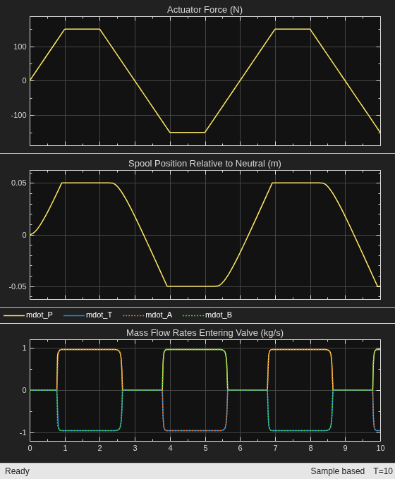
Actuate the valve by first applying a force of 150 N to move the spool in the positive direction, then a force of -150 N to move the spool in the negative direction. When the spool moves in the positive direction, paths P-B and A-T open, causing fluid to flow from B to A through the load. When the spool moves in the negative direction, paths P-A and B-T open, causing fluid to flow from A to B through the load.

Simulate the model and observe the results in the scope. The spool position moves to 0.05 m relative to neutral when a positive force is applied, then to -0.05 m relative to neutral when a negative force is applied. Note that 0.05 m is the value of L_gap calculated above. The mass flow rates measurements mdot_P, mdot_T, mdot_A, and mdot_B are set up to be positive when the fluid flow enters the valve. When paths P-B and A-T are open, mdot_P and mdot_A are positive while mdot_T and mdot_B are negative. When paths P-A and B-T are open, mdot_P and mdot_B are positive while mdot_T and mdot_A are negative. Furthermore, because the valve is overlapped, the flow rate is zero when the spool is near the neutral position.

open_system(model + "/Scope")
sim(model)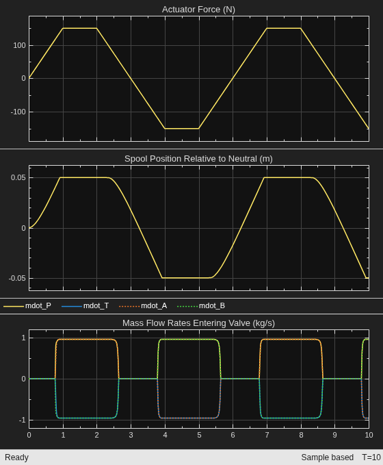

Using the logged data, you can plot the opening distance and the metering area for the various valve port and spool land combinations. The opening distance is the distance between the land edge and the valve port edge. The block defines the value of zero to be when the two edges are on top of each other. The metering area is the area between the land edge and the valve port edge that restricts fluid flow. As the opening distance increases, the metering area increases to permit more flow.

Examine the block Valve Port with Land Edge (IL-PB) - Left. It has two metering areas and two corresponding opening distances because there is a flow path through the valve port to either the left side of the land (side B) or the right side of the land (side F). First, extract the desired simulation results from the logged data:

t = simlog_Hydromechanical4WayDirectionalValve.Valve_Port_with_Land_IL_PB_Left.opening_B.series.time;
opening_left  = simlog_Hydromechanical4WayDirectionalValve.Valve_Port_with_Land_IL_PB_Left.opening_B.series.values("m");
opening_right = simlog_Hydromechanical4WayDirectionalValve.Valve_Port_with_Land_IL_PB_Left.opening_F.series.values("m");
area_left  = simlog_Hydromechanical4WayDirectionalValve.Valve_Port_with_Land_IL_PB_Left.metering_area_B.series.values("m^2");
area_right = simlog_Hydromechanical4WayDirectionalValve.Valve_Port_with_Land_IL_PB_Left.metering_area_F.series.values("m^2");

Next, generate the plot:

figure
tiledlayout(2, 1)
ax(1) = nexttile;
plot(t, opening_left, t, opening_right, LineWidth = 1)
grid on
title("Valve Port with Land Edge (IL-PB) - Left")
ylabel("Opening Distance (m)")
legend("Left Side of Land (Side B)", "Right Side of Land (Side F)", Location = "southoutside", Orientation = "horizontal")
ax(2) = nexttile;
plot(t, area_left, t, area_right, LineWidth = 1)
grid on
ylabel("Metering Area (m^2)")
xlabel("Time (s)")
linkaxes(ax, "x")

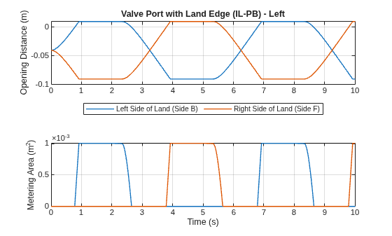
Figure contains 2 axes objects. Axes object 1 with title Valve Port with Land Edge (IL-PB) - Left, ylabel Opening Distance (m) contains 2 objects of type line. These objects represent Left Side of Land (Side B), Right Side of Land (Side F). Axes object 2 with xlabel Time (s), ylabel Metering Area (m^2) contains 2 objects of type line.

The metering area of each side remain closed until the corresponding opening distance rises above 0 m. In this model, the opening distances do not reach the full valve port width of W_port = 0.02 m. Therefore, the metering areas do not reach the full valve port area of W_port * L_port = 2e-3 m^2.

Examine the block Valve Section with Valve Port (IL-PB) - Middle. It has one metering area because there is only one flow path through the valve port to the space between the two adjacent lands. However, it has two opening distances because the metering area can be blocked by either the adjacent land coming from the left side (side B) or the adjacent land coming from the right side (side F). First, extract the desired simulation results from the logged data:

t = simlog_Hydromechanical4WayDirectionalValve.Valve_Section_with_Valve_Port_IL_PB_Middle.opening_B.series.time;
opening_left  = simlog_Hydromechanical4WayDirectionalValve.Valve_Section_with_Valve_Port_IL_PB_Middle.opening_B.series.values("m");
opening_right = simlog_Hydromechanical4WayDirectionalValve.Valve_Section_with_Valve_Port_IL_PB_Middle.opening_F.series.values("m");
area = simlog_Hydromechanical4WayDirectionalValve.Valve_Section_with_Valve_Port_IL_PB_Middle.metering_area.series.values("m^2");

Next, generate the plot:

figure
tiledlayout(2, 1)
ax(1) = nexttile;
plot(t, opening_left, t, opening_right, LineWidth = 1)
grid on
title("Valve Section with Valve Port (IL-PB) - Middle")
ylabel("Opening Distance (m)")
legend("Land from Left Side (Side B)", "Land from Right Side (Side F)", Location = "southoutside", Orientation = "horizontal")
ax(2) = nexttile;
plot(t, area, LineWidth = 1)
grid on
ylabel("Metering Area (m^2)")
xlabel("Time (s)")
linkaxes(ax, "x")

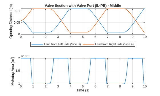
Figure contains 2 axes objects. Axes object 1 with title Valve Section with Valve Port (IL-PB) - Middle, ylabel Opening Distance (m) contains 2 objects of type line. These objects represent Land from Left Side (Side B), Land from Right Side (Side F). Axes object 2 with xlabel Time (s), ylabel Metering Area (m^2) contains an object of type line.

The metering area remains fully open at the valve port area of W_port * L_port = 2e-3 m^2 until one of the two opening distances fall below the valve port width of W_port = 0.02 m. This illustrates how the metering behavior of a Valve Section with Valve Port (IL-PB) block is opposite to the metering behavior of a Valve Port with Land (IL-PB) block.

Mechanical Forces

The force input applied to the spool moves the spool towards the left end cap or the right end cap. When the spool hits either end caps, a hard stop engages to limit the motion of the spool. In addition, springs at the two end caps push the spool back to the neutral center position. To see these forces, first extract the simulation results from the Valve Section with End Cap at B (IL-PB) block and the Valve Section with End Cap at F (IL-PB) block:

t = simlog_Hydromechanical4WayDirectionalValve.Valve_Section_with_End_Cap_at_B_IL_PB.gap_length.series.time;
gap_length_left  = simlog_Hydromechanical4WayDirectionalValve.Valve_Section_with_End_Cap_at_B_IL_PB.gap_length.series.values("m");
gap_length_right = simlog_Hydromechanical4WayDirectionalValve.Valve_Section_with_End_Cap_at_F_IL_PB.gap_length.series.values("m");
f_spring_left  = simlog_Hydromechanical4WayDirectionalValve.Valve_Section_with_End_Cap_at_B_IL_PB.f_spring.series.values("N");
f_spring_right = simlog_Hydromechanical4WayDirectionalValve.Valve_Section_with_End_Cap_at_F_IL_PB.f_spring.series.values("N");
f_hardstop_left  = simlog_Hydromechanical4WayDirectionalValve.Valve_Section_with_End_Cap_at_B_IL_PB.f_hardstop.series.values("N");
f_hardstop_right = simlog_Hydromechanical4WayDirectionalValve.Valve_Section_with_End_Cap_at_F_IL_PB.f_hardstop.series.values("N");

Plot the spring forces:

figure
tiledlayout(2, 1)
ax(1) = nexttile;
plot(t, gap_length_left, t, gap_length_right, LineWidth = 1)
grid on
title("Distance Between End Cap and Spool")
ylabel("Gap Length (m)")
legend("Left End Cap", "Right End Cap", Location = "southoutside", Orientation = "horizontal")
ax(2) = nexttile;
plot(t, f_spring_left, t, f_spring_right, LineWidth = 1)
grid on
title("Spring Force")
ylabel("Force (N)")
xlabel("Time (s)")
linkaxes(ax, "x")

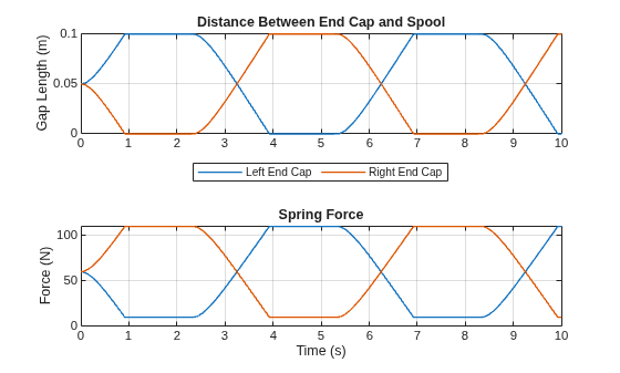
Figure contains 2 axes objects. Axes object 1 with title Distance Between End Cap and Spool, ylabel Gap Length (m) contains 2 objects of type line. These objects represent Left End Cap, Right End Cap. Axes object 2 with title Spring Force, xlabel Time (s), ylabel Force (N) contains 2 objects of type line.

The gap_length variable at the end cap valve sections is the distance between the end cap and the spool. The springs start at a preload force of 60 N. As the spool moves to the right, the gap length at the left end cap increases and the gap length at the right end cap decreases, causing the spring force at the left end cap to decrease and the spring force at the right end cap to increase. As the spool moves to the left, the reverse happens.

Next, plot the hard stop forces:

figure
tiledlayout(2, 1)
ax(1) = nexttile;
plot(t, gap_length_left, t, gap_length_right, LineWidth = 1)
grid on
title("Distance Between End Cap and Spool")
ylabel("Gap Length (m)")
legend("Left End Cap", "Right End Cap", Location = "southoutside", Orientation = "horizontal")
ax(2) = nexttile;
plot(t, f_hardstop_left, t, f_hardstop_right, LineWidth = 1)
grid on
title("Hard Stop Force")
ylabel("Force (N)")
xlabel("Time (s)")
linkaxes(ax, "x")

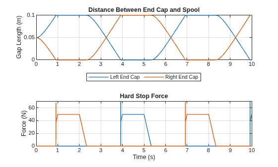
Figure contains 2 axes objects. Axes object 1 with title Distance Between End Cap and Spool, ylabel Gap Length (m) contains 2 objects of type line. These objects represent Left End Cap, Right End Cap. Axes object 2 with title Hard Stop Force, xlabel Time (s), ylabel Force (N) contains 2 objects of type line.

The hard stop forces remain at zero until the gap length reaches zero. At that point, there is a sudden increase and spike in the hard stop force because it needs to counteract the inertial force due to the mass of the moving spool when bringing the spool to a stop. After the spool is stopped, the hard stop force only needs to counteract further increases in the force input to keep the spool at rest.

Mass and Damping Effects

You can model the dynamic response of the spool by enabling spool mass and damping effects in the Valve Port with Land (IL-PB) blocks or the Valve Piston (IL-PB) blocks. Some scenarios also require you to enable mass and/or damping to simulate the model robustly. A valve with force input is one such scenario.

The example model Hydromechanical4WayDirectionalValve is already configured with mass and damping enabled to produce all of the above simulation results. However, the hydromechanical valve blocks do not have mass and damping enabled by default. To see what happens if you leave mass and damping disabled, turn it off in the example model and simulate:

set_param(model + "/Valve Port with Land (IL-PB) - Left", "enable_land_mass", "false")
set_param(model + "/Valve Port with Land (IL-PB) - Left", "enable_damping", "false")
set_param(model + "/Valve Port with Land (IL-PB) - Right", "enable_land_mass", "false")
set_param(model + "/Valve Port with Land (IL-PB) - Right", "enable_damping", "false")

try
    sim(model)
catch ME
    disp(ME)
    disp(ME.cause{1})
    disp(ME.cause{1}.cause{1})
end

  MSLException with properties:

       handles: {[474.0026]}
    identifier: 'physmod:simscape:engine:core:dae_errors:NE_DAE_IC_Failure'
       message: '['Hydromechanical4WayDirectionalValve/Solver Configuration']: Initial conditions solve failed to converge.'
         cause: {[1×1 MSLException]}
         stack: [7×1 struct]
    Correction: []

  MSLException with properties:

       handles: {[0×1 double]}
    identifier: 'physmod:simscape:engine:core:dae_errors:NE_DAE_nlsolve_NE_LA_Solve_Failure'
       message: 'Nonlinear solver: Linear Algebra error. Failed to solve using iteration matrix.'
         cause: {[1×1 MSLException]}
         stack: [7×1 struct]
    Correction: []

  MSLException with properties:

       handles: {[0×1 double]}
    identifier: 'physmod:simscape:engine:core:dae_errors:NE_DAE_dependency_diagnostic'
       message: 'all components and nodal across variables involved↵Cannot solve for one or more variables, including dynamic variable derivatives:↵Time derivative of 'External_Force_Source_PB.R.x' (Position)↵Time derivative of 'Valve_Piston_IL_PB_Left.F.spool.x' (Position)↵Time derivative of 'Valve_Piston_IL_PB_Right.F.spool.x' (Position)↵Time derivative of 'Valve_Port_with_Land_IL_PB_Left.F.spool.x' (Position)↵Time derivative of 'Valve_Port_with_Land_IL_PB_Right.F.spool.x' (Position)↵Time derivative of 'Valve_Section_with_End_Cap_at_B_IL_PB.Bs.x' (Position)↵Time derivative of 'Valve_Section_with_End_Cap_at_F_IL_PB.Fs.x' (Position)↵Time derivative of 'Valve_Piston_IL_PB_Left.B.spool.x' (Position)↵Time derivative of 'Valve_Piston_IL_PB_Right.B.spool.x' (Position)↵Time derivative of 'Valve_Port_with_Land_IL_PB_Left.B.spool.x' (Position)↵Time derivative of 'Valve_Port_with_Land_IL_PB_Right.B.spool.x' (Position)↵'External_Force_Source_PB.R.v' (Velocity)↵'Valve_Piston_IL_PB_Left.F.spool.v' (Velocity)↵'Valve_Piston_IL_PB_Left.piston.B.v' (Velocity)↵'Valve_Piston_IL_PB_Left.piston.F.v' (Velocity)↵'Valve_Piston_IL_PB_Right.F.spool.v' (Velocity)↵<a href="matlab:simscape.internal.highlightSLStudio({'Hydromechanical4WayDirectionalValve/Valve Piston (IL-PB) - Right'}, {''})">'Valv…'         cause: {}
         stack: [7×1 struct]
    Correction: []

The error message indicates that the solver failed to initialize the model because it cannot solve for the derivatives of some of the dynamic variables. The error occurs because the model uses force actuation to move the spool, but there is no mass for the force to push on, resulting in infinite acceleration.

To address this issue, enable mass in the spool land. Because the lands and shafts are all rigidly connected, you can lump the entire spool's mass into a single value for any one of the lands. Alternatively, you can distribute the spool mass by enabling mass in multiple lands. The solver will internally sum the mass of all rigidly connected lands.

M_spool = 0.5; % kg
set_param(model + "/Valve Port with Land (IL-PB) - Left", "enable_land_mass", "true")
set_param(model + "/Valve Port with Land (IL-PB) - Left", "land_mass", "M_spool")

When you enable mass, the velocity of the spool land relative to the valve body becomes a differential variable that requires an initial condition. Set a high priority target value of 0 m/s:

set_param(model + "/Valve Port with Land (IL-PB) - Left", "v_rel_land_specify", "on")
set_param(model + "/Valve Port with Land (IL-PB) - Left", "v_rel_land_priority", "high")
set_param(model + "/Valve Port with Land (IL-PB) - Left", "v_rel_land", "0")

Simulate the model and observe the results in the scope.

open_system(model + "/Scope")
sim(model)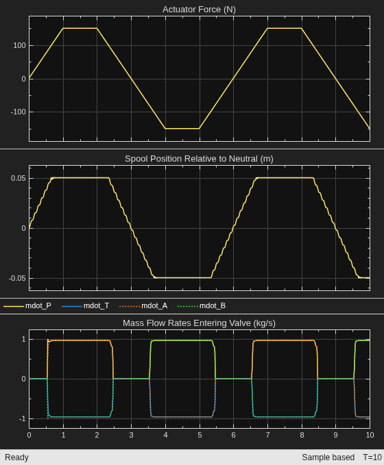

While the model simulates successfully, there are now oscillations in the spool position. These oscillations can affect the metering areas and flow rates. The oscillations occur because the model is now a second order spring-mass system without damping.

To remove the oscillations, enable damping between the spool and the valve body. The damping is modeled as viscous friction due to the fluid trapped in the clearance between the spool lands and the valve body.

h_clearance = 5e-6; % m
set_param(model + "/Valve Port with Land (IL-PB) - Left", "enable_damping", "true")
set_param(model + "/Valve Port with Land (IL-PB) - Left", "land_diameter", "D_land_outer")
set_param(model + "/Valve Port with Land (IL-PB) - Left", "radial_clearance", "h_clearance")
set_param(model + "/Valve Port with Land (IL-PB) - Right", "enable_damping", "true")
set_param(model + "/Valve Port with Land (IL-PB) - Right", "land_diameter", "D_land_outer")
set_param(model + "/Valve Port with Land (IL-PB) - Right", "radial_clearance", "h_clearance")

Simulate the model and observe that the damping has suppressed the oscillations.

open_system(model + "/Scope")
sim(model)