Hydromechanical Poppet Check Valve

R2026b

Since R2026b

This example shows how to build a check valve with a poppet design using components from the Hydromechanical Valves library and compares it to the behavioral Check Valve (IL) block.

model = "HydromechanicalPoppetCheckValve";
open_system(model)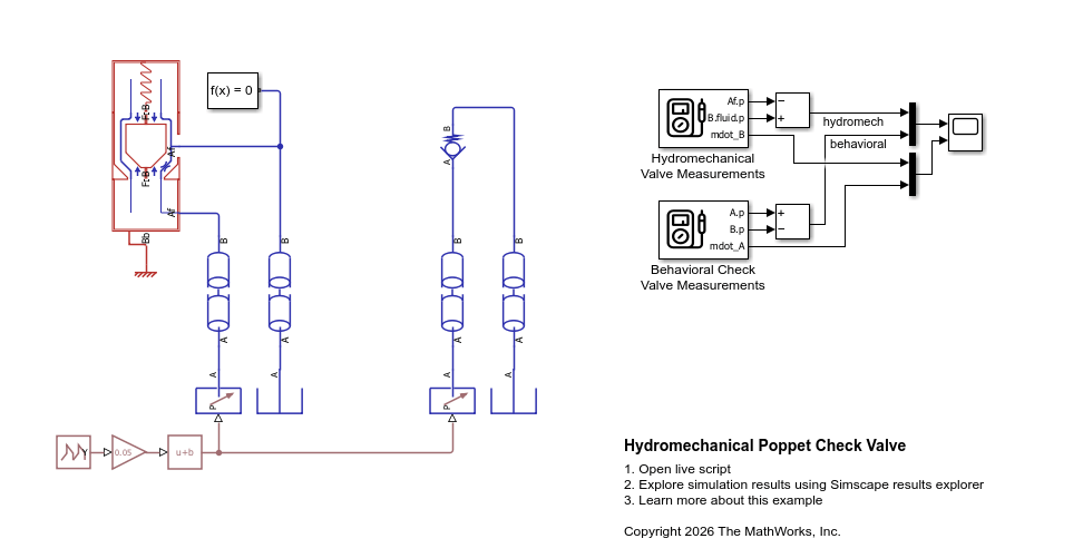

Model Overview

Each block in the Hydromechanical Valves library models a piece of a valve that you combine to model a complete valve. The block icons are intended to be arranged next to each other to resemble a valve schematic, but they must still be connected together via their B and F hydromechanical valve ports. The figure below shows the model with the individual blocks identified and spaced apart to show the connection lines.

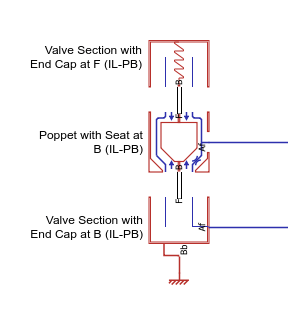
The check valve model consists of the following hydromechanical valve blocks:

Valve Section with End Cap at B (IL-PB) - models the fluid chamber in front of the valve seat and provides the isothermal liquid connection for the fluid to enter the valve structure.
Poppet with Seat at B (IL-PB) - models the valve seat and poppet mechanism that meters flow through the valve seat.
Valve Section with End Cap at F (IL-PB) - models the fluid chamber that the poppet can move into when it is pushed off the valve seat as well as the spring that returns the poppet to the valve seat.

For more information, see Get Started with the Hydromechanical Valve Library.

Model Setup

The model HydromechanicalPoppetCheckValve is already fully configured and ready to simulate a check valve. This section highlights the key steps in configuring the model.

The fluid enters the valve structure via port Af in Valve Section with End Cap at B (IL-PB) block. This port provides a direct isothermal liquid network connection to the fluid inside the valve. To model this connection, configure the bottom end cap valve section to contain liquid and to expose the isothermal liquid port Af:

set_param(model + "/Valve Section with End Cap at B (IL-PB)", "contains_liquid", "true")
set_param(model + "/Valve Section with End Cap at B (IL-PB)", "enable_liquid_port", "true")

Once the fluid is inside the valve, it flows through the valve port and is metered by the poppet. The metered flow then leaves the valve while some of the fluid wraps around the poppet to the end cap valve section behind the poppet.

set_param(model + "/Poppet with Seat at B (IL-PB)", "contains_liquid_F", "true")

There is no outlet for the fluid in the top end cap valve section so do not expose its isothermal liquid port Af. The fluid is simply there to apply a pressure force on the poppet.

set_param(model + "/Valve Section with End Cap at F (IL-PB)", "contains_liquid", "true")
set_param(model + "/Valve Section with End Cap at F (IL-PB)", "enable_liquid_port", "false")

Note that if you do not set contains_liquid to true in the two end cap valve sections, the icons do not show the blue isothermal liquid lines, signifying that there is no fluid inside. Therefore, the blue lines in the poppet with seat block will not match up with any blue lines in the adjacent valve section blocks. This mismatch in adjacent icons is a visual indication that the model is not configured correctly.

Unlike a spool valve, the poppet is not externally actuated. Instead, it moves based on the net pressure force on the poppet. In addition, a spring keeps the poppet seated against the valve seat until the pressure force is large enough to overcome the spring force. Enable the spring in the top end cap valve section to model the spring force acting on the poppet.

set_param(model + "/Valve Section with End Cap at F (IL-PB)", "enable_spring", "true")

All mechanical models, including hydromechanical valve models, need a reference point to define the zero position. In this model, the bottom end cap is the reference position. Therefore, expose the position-based translational port Bb for the valve body and connect it to the Translational World (PB) block.

set_param(model + "/Valve Section with End Cap at B (IL-PB)", "enable_cap_port", "true")

Model Parameters

After configuring the model, parameterize the blocks to define the spacing between the end caps, the valve seat, and the poppet. The spacing provides information on how far the poppet can move and the fluid volume available on either side of the poppet as it moves.

Model the contact surface of both the poppet and the valve seat as conical with a 120 deg cone angle:

theta_poppet = 120; % deg
set_param(model + "/Poppet with Seat at B (IL-PB)", "poppet_cone_angle", "theta_poppet")

The maximum flow area is the area of the valve seat. Assume that the fluid chamber in the valve section on the other side of the valve seat has the same area.

D_seat = 0.07; % m
A_seat = pi*D_seat^2/4

A_seat = 
0.0038

set_param(model + "/Poppet with Seat at B (IL-PB)", "seat_diameter", "D_seat")
set_param(model + "/Valve Section with End Cap at B (IL-PB)", "section_area", "pi*D_seat^2/4")

The two end cap valve section blocks define the distance between the end caps and the valve seat. Assume that the valve seat is located in the middle of the valve.

L_body = 0.1; % m
set_param(model + "/Valve Section with End Cap at B (IL-PB)", "body_length", "L_body")
set_param(model + "/Valve Section with End Cap at F (IL-PB)", "body_length", "L_body")

Although the poppet diameter is not needed to calculate the metering area for a conical poppet geometry, assume that the fluid chamber in the top end cap valve section has an area based on the poppet diameter.

D_poppet = 0.1; % m
A_poppet = pi*D_poppet^2/4

A_poppet = 
0.0079

set_param(model + "/Valve Section with End Cap at F (IL-PB)", "section_area", "pi*D_poppet^2/4")

In addition, the top end cap valve section contains a spring that pushes the poppet against the valve seat. Tune the spring such that the valve requires a certain amount of cracking pressure in order to unseat the poppet. Specify the reference spring force based on the cracking pressure:

k_spring = 3000; % N/m
p_crack = 0.015 * 1e6; % Pa
f_spring_ref = p_crack * (pi*D_seat^2/4)

f_spring_ref = 
57.7268

set_param(model + "/Valve Section with End Cap at F (IL-PB)", "spring_stiffness", "k_spring")
set_param(model + "/Valve Section with End Cap at F (IL-PB)", "spring_force_ref", "p_crack * (pi*D_seat^2/4)")

The cracking pressure force is applied when the poppet is seated, so the reference spring length corresponding to the reference spring force is the difference between the end cap section length and the poppet length:

L_poppet = 0.05; % m
set_param(model + "/Valve Section with End Cap at F (IL-PB)", "gap_length_ref", "L_body - L_poppet")

Finally, specify the area of the fluid channels connected to the valve, which refers to the area of the outer valve ports or external pipes. While the hydromechanical valve blocks do not model these fluid channels themselves, the purpose of this parameter is to provide some pressure loss even when the poppet is fully lifted from the valve seat based on the area ratio of the valve seat to the connecting fluid channels.

A_conn = 0.005; % m^2
set_param(model + "/Poppet with Seat at B (IL-PB)", "connecting_area", "A_conn")

Simulate with Pressure Input

Simulate the valve behavior by varying the pressure of the upstream reservoir as a function of time. The upstream pressure first rises above the downstream pressure and then falls below the downstream pressure. When the difference between the upstream and downstream pressure reaches the cracking pressure, the poppet moves away from the valve seat and permit fluid flow. Otherwise, the poppet remains seated and blocks fluid flow.

Provide an initial condition for the poppet position by assigning a high priority initial target value to the valve_lift variable. This value corresponds with an initial spring deformation and thus an initial spring force, which is balanced by the initial pressures in the two end cap valve sections.

lift_init = 0; % m
set_param(model + "/Poppet with Seat at B (IL-PB)", "lift_specify", "on")
set_param(model + "/Poppet with Seat at B (IL-PB)", "lift_priority", "High")
set_param(model + "/Poppet with Seat at B (IL-PB)", "lift", "lift_init")

Simulate the model and observe the results in the scope. This model uses the Simscape Probe to measure the results. Because the hydromechanical valve ports B and F are composed of three separate Simscape networks, you need to access the pressure at port B as B.fluid.p. Port Af is a regular isothermal liquid valve port so its pressure is simply Af.p.

open_system(model + "/Scope")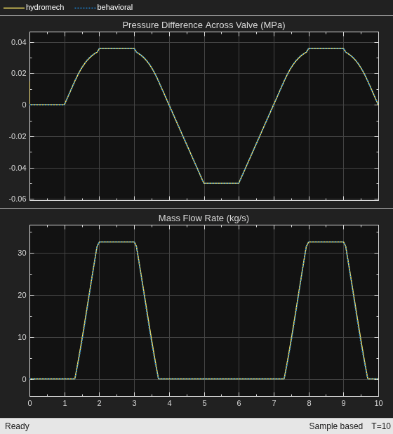

sim(model)

The simulation results show that there is positive flow through the valve when the pressure difference is above the cracking pressure of 0.015 MPa. During this period, the pressure difference does not rise significantly above the cracking pressure because the poppet is away from the seat and the flow is relatively unrestricted. When the pressure difference falls below the cracking pressure, the flow stops, and the pressure difference continues to fall.

Using the logged data, plot the valve lift and the metering area. The valve lift is the distance between the poppet and the valve seat. The block defines the value of zero to be when the poppet is just touching the valve seat. The Poppet with Seat at B (IL-PB) block models a hard stop between the poppet and the valve seat. Because the hard stop stiffness is not infinite, the valve lift can be slightly negative. The metering area is the frustum area between the poppet and the valve seat. As the valve lift increases, the metering area increases to permit more flow through the valve seat.

First, extract the desired simulation results from the logged data:

t = simlog_HydromechanicalPoppetCheckValve.Poppet_with_Seat_at_B_IL_PB.lift.series.time;
valve_lift = simlog_HydromechanicalPoppetCheckValve.Poppet_with_Seat_at_B_IL_PB.lift.series.values("m");
metering_area = simlog_HydromechanicalPoppetCheckValve.Poppet_with_Seat_at_B_IL_PB.metering_area.series.values("m^2");

Next, generate the plot:

figure
tiledlayout(2, 1)
ax(1) = nexttile;
plot(t, valve_lift, LineWidth = 1)
grid on
title("Valve Lift")
ylabel("Valve Lift (m)")
ax(2) = nexttile;
plot(t, metering_area, LineWidth = 1)
grid on
title("Metering Area")
ylabel("Metering Area (m^2)")
xlabel("Time (s)")
linkaxes(ax, "x")

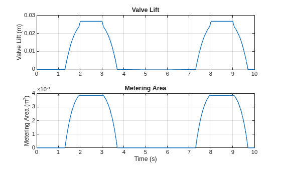
Figure contains 2 axes objects. Axes object 1 with title Valve Lift, ylabel Valve Lift (m) contains an object of type line. Axes object 2 with title Metering Area, xlabel Time (s), ylabel Metering Area (m^2) contains an object of type line.

The plot shows that as the valve lift increases, there comes a point where the metering area saturates at the maximum area equal to the valve seat area.

A_seat

A_seat = 
0.0038

After this point, there is a bump in the valve lift plot. The bump occurs because the upstream pressure continues to rise for a short moment after the metering area reached its maximum. Because the metering area cannot increase any further to relieve the pressure, there is a bump in the pressure difference and a corresponding bump in the valve lift.

Comparison to Behavioral Check Valve

The Hydromechanical Valves library lets you build up complex customized valves based on the geometry of the valve structure. Other blocks in the Valves & Orifices library are behavioral components because they model the behavior of the valve without considering the detailed geometry and mechanical effects of the valve structure. For common valve configurations, the more detailed hydromechanical valve model and the simpler behavioral valve model can produce the same results. This example compares the hydromechanical poppet check valve to the behavioral Check Valve (IL) block and shows how the geometrical parameters of the hydromechanical valve map to the behavioral valve.

The behavioral valve does not model valve lift. Instead, the block calculates the valve area directly based on the pressure difference. You know the cracking pressure value, but need to determine the maximum pressure. The maximum pressure occurs when the metering area reaches its maximum value of the valve seat area. At this point, the poppet will be at a location denoted as lift_max. The spring force that corresponds to lift_max will be the maximum pressure force.

The value of lift_max depends on the geometry of the poppet and the valve seat. You can see the characteristics of the specified geometry by plotting the metering area versus valve lift using the Plot button on the Poppet with Seat at B (IL-PB) dialog. The valve lift that corresponds to the maximum metering area is reported in this plot.

fluids.internal.mask.plotHydromechMeteringAreaPoppet(model + "/Poppet with Seat at B (IL-PB)")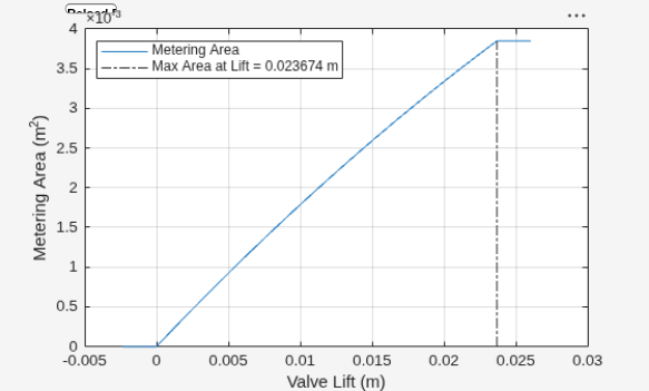

Figure Poppet with Seat at B (IL-PB) contains an axes object and another object of type uicontrol. The axes object with xlabel Valve Lift (m), ylabel Metering Area (m Squared baseline ) contains 2 objects of type line. These objects represent Metering Area, Max Area at Lift = 0.023674 m.

lift_max = 0.023674; % m

The maximum pressure is then

p_max = (lift_max * k_spring)/(pi*D_seat^2/4) + p_crack

p_max = 
3.3455e+04

set_param(model + "/Check Valve (IL)", "p_crack_differential", "p_crack")
set_param(model + "/Check Valve (IL)", "press_max_differential", "(lift_max * k_spring)/(pi*D_seat^2/4) + p_crack")

The maximum area is the valve seat area and the minimum area is (by default in the hydromechanical valve) a factor of 1e-6 smaller:

set_param(model + "/Check Valve (IL)", "area_max", "pi*D_seat^2/4")
set_param(model + "/Check Valve (IL)", "area_leak", "1e-6 * (pi*D_seat^2/4)")

The cross-sectional area at ports A and B of the behavioral valve is equivalent to the area of the fluid channels connected to the hydromechanical valve:

set_param(model + "/Check Valve (IL)", "area", "A_conn")

Simulate the model and observe the results in the scope. The results show that the pressure differences and the mass flow rates for the behavioral valve and the hydromechanical valve are very close using the parameter mapping above.

open_system(model + "/Scope")
sim(model)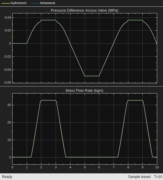

You can also use the logged data to compare the metering areas. First, extract the simulation results for the hydromechanical valve and the behavioral valve:

t = simlog_HydromechanicalPoppetCheckValve.Poppet_with_Seat_at_B_IL_PB.metering_area.series.time;
metering_area = simlog_HydromechanicalPoppetCheckValve.Poppet_with_Seat_at_B_IL_PB.metering_area.series.values("m^2");
mdot = simlog_HydromechanicalPoppetCheckValve.Poppet_with_Seat_at_B_IL_PB.mdot_B.series.values("kg/s");

metering_area_behavioral = simlog_HydromechanicalPoppetCheckValve.Check_Valve_IL.valve_area.series.values("m^2");
mdot_behavioral = simlog_HydromechanicalPoppetCheckValve.Check_Valve_IL.mdot_A.series.values("kg/s");

Next, generate the plot:

figure
tiledlayout(2, 1)
ax(1) = nexttile;
plot(t, metering_area, "-", t, metering_area_behavioral, "--", LineWidth = 1)
hold off
grid on
title("Metering Area")
ylabel("Metering Area (m^2)")
legend("Hydromechanical", "Behavioral", Location = "southoutside", Orientation = "horizontal")
ax(2) = nexttile;
plot(t, mdot, "-", t, mdot_behavioral, "--", LineWidth = 1)
hold off
grid on
title("Mass Flow Rate")
ylabel("Mass Flow Rate (kg/s)")
xlabel("Time (s)")
linkaxes(ax, "x")

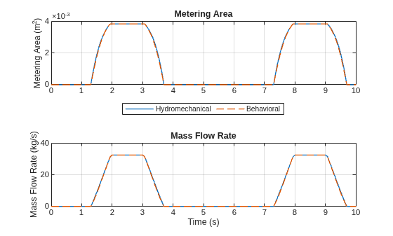
Figure contains 2 axes objects. Axes object 1 with title Metering Area, ylabel Metering Area (m^2) contains 2 objects of type line. These objects represent Hydromechanical, Behavioral. Axes object 2 with title Mass Flow Rate, xlabel Time (s), ylabel Mass Flow Rate (kg/s) contains 2 objects of type line.

The metering areas and the mass flow rates match between the hydromechanical valve and the behavioral valve.

Poppet Mass Dynamic Response

The hydromechanical check valve allows you to simulate the dynamic response of the valve based on the net force on the poppet, which is not available in the behavioral check valve block. Start by enabling the poppet mass, which allows the block to model the acceleration of the poppet:

M_poppet = 3; % kg
set_param(model + "/Poppet with Seat at B (IL-PB)", "enable_poppet_mass", "true")
set_param(model + "/Poppet with Seat at B (IL-PB)", "poppet_mass", "M_poppet")

Modeling the poppet mass means that the block has an additional differential state for the poppet velocity, which requires an additional initial condition. The simplest initial condition is to set the initial velocity to zero:

set_param(model + "/Poppet with Seat at B (IL-PB)", "v_rel_poppet_specify", "on")
set_param(model + "/Poppet with Seat at B (IL-PB)", "v_rel_poppet_priority", "High")
set_param(model + "/Poppet with Seat at B (IL-PB)", "v_rel_poppet", "0")

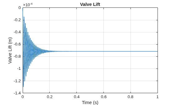
Simulate the model and observe the results in the scope. The results show that the relatively large mass and the spring results in some oscillations.

open_system(model + "/Scope")
sim(model)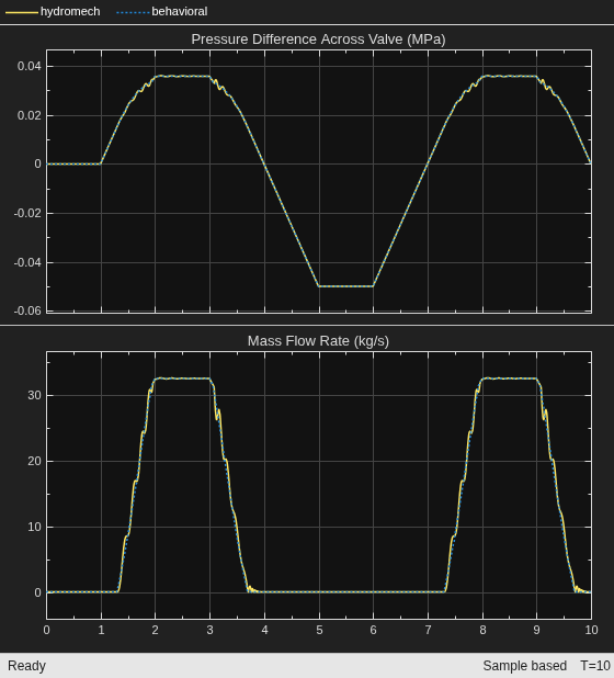

If you zoom in to the valve lift near the start of the simulation, you can see that it is oscillating before settling down. The oscillations are due to a force imbalance on the poppet at the initial valve lift of zero.

t = simlog_HydromechanicalPoppetCheckValve.Poppet_with_Seat_at_B_IL_PB.lift.series.time;
valve_lift = simlog_HydromechanicalPoppetCheckValve.Poppet_with_Seat_at_B_IL_PB.lift.series.values("m");

figure
plot(t, valve_lift, LineWidth = 1)
grid on
title("Valve Lift")
ylabel("Valve Lift (m)")
xlabel("Time (s)")
xlim([0, 1])

Figure contains an axes object. The axes object with title Valve Lift, xlabel Time (s), ylabel Valve Lift (m) contains an object of type line.

If the initial oscillations are undesirable, you can change the initial conditions on the poppet to have no initial acceleration.

set_param(model + "/Poppet with Seat at B (IL-PB)", "f_acc_poppet_specify", "on")
set_param(model + "/Poppet with Seat at B (IL-PB)", "f_acc_poppet_priority", "High")
set_param(model + "/Poppet with Seat at B (IL-PB)", "f_acc_poppet", "0")

However, because you added an additional initial condition, you have to remove one to avoid overconstraining the initial equations. Remove the initial target on the valve lift and thus reverting it to the default setting of none priority.

set_param(model + "/Poppet with Seat at B (IL-PB)", "lift_specify", "off")

Simulate the model again and replot the valve lift near the start of the simulation.

close_system(model + "/Scope")
sim(model)

t = simlog_HydromechanicalPoppetCheckValve.Poppet_with_Seat_at_B_IL_PB.lift.series.time;
valve_lift = simlog_HydromechanicalPoppetCheckValve.Poppet_with_Seat_at_B_IL_PB.lift.series.values("m");

figure
plot(t, valve_lift, LineWidth = 1)
grid on
title("Valve Lift")
ylabel("Valve Lift (m)")
xlabel("Time (s)")
xlim([0, 1])
ylim([-1e-4 1e-4])

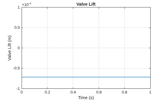
Figure contains an axes object. The axes object with title Valve Lift, xlabel Time (s), ylabel Valve Lift (m) contains an object of type line.

The plot shows that the valve now starts the simulation in its own local steady-state.

Pressure Difference Versus Gauge Pressure

The hydromechanical check valve is currently configured to open based on the pressure difference across the poppet. You can also configure it to open based on the gauge pressure on the valve seat side of the poppet. To simulate this configuration, first reset the model to the way it was without the poppet mass.

set_param(model + "/Poppet with Seat at B (IL-PB)", "enable_poppet_mass", "false")
set_param(model + "/Poppet with Seat at B (IL-PB)", "lift_specify", "on")

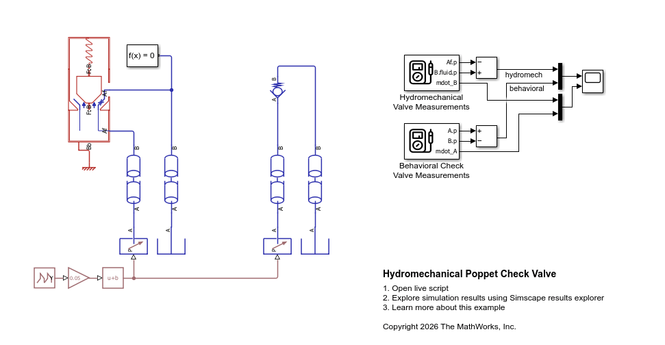
For the poppet to open based on gauge pressure, the top end cap valve section should be open to the atmosphere. Disable the option to let the liquid flow around the poppet because the back of the poppet is now open to the atmosphere.

set_param(model + "/Valve Section with End Cap at F (IL-PB)", "contains_liquid", "false")
set_param(model + "/Poppet with Seat at B (IL-PB)", "contains_liquid_F", "false")

The figure below shows that the blue isothermal liquid lines in the block icons no longer wraps around the poppet to the top end cap valve section.

Configure the behavioral check valve to open based on gauge pressure at port A and with the same cracking and maximum pressure settings:

set_param(model + "/Check Valve (IL)", "pressure_control_spec", ...
    "fluids.isothermal_liquid.valves_orifices.enum.pressure_control_spec.pA")
set_param(model + "/Check Valve (IL)", "p_crack_gauge", "p_crack")
set_param(model + "/Check Valve (IL)", "press_max_gauge", "(lift_max * k_spring)/(pi*D_seat^2/4) + p_crack")

Simulate the model and observe the results in the scope. The results show that the valve now has a slightly different opening characteristic.

open_system(model + "/Scope")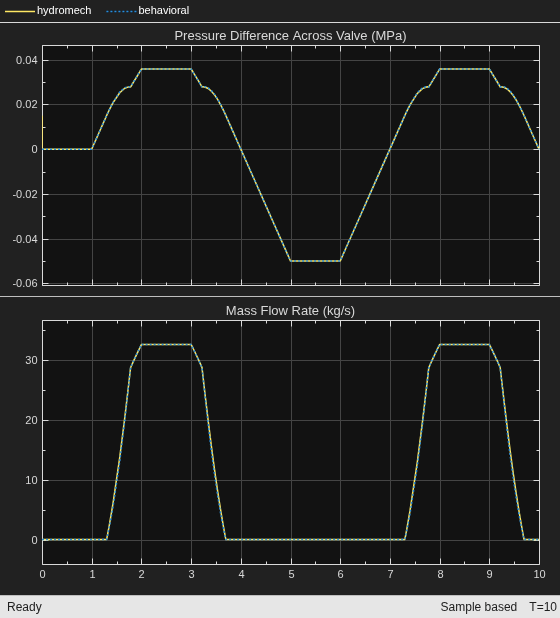

sim(model)