Analyze Time Series Data Using Econometric Modeler
The Econometric Modeler app is an interactive tool for analyzing univariate or multivariate time series data. The app is well suited for visualizing and transforming data, performing statistical specification and model identification tests, fitting models to data and comparing their fit statistics, simulating and forecasting models, and iterating among these actions. When you are satisfied with a model, you can export it to the MATLAB® Workspace to forecast future responses or for further analysis. You can also generate code or a report from a session.
Start Econometric Modeler by entering econometricModeler at the
MATLAB command line, or by clicking Econometric Modeler
under Computational Finance in the apps gallery
(Apps tab on the MATLAB Toolstrip).
The following workflow describes how to find a model with the best in-sample fit to time series data, and then forecast the best model, using Econometric Modeler. The workflow is not a strict prescription—the steps you implement depend on your goals and the model type. You can easily skip steps and iterate several steps as needed. The app is well suited to the Box-Jenkins approach to time series model building [1].
Prepare data for Econometric Modeler — For a response variable, or select multiple response variables for a multivariate analysis, to analyze and from which to build a predictive model. Optionally, select explanatory variables to include in the model.
Note
You can import only one variable from the MATLAB Workspace into Econometric Modeler. Therefore, at the command line, you must synchronize and concatenate multiple series into one variable.
Configure Econometric Modeler — Specify the look and behavior of the app.
Import time series variables — Import Data into Econometric Modeler from the MATLAB Workspace or a MAT-file. After importing data, you can adjust variable properties or the presence of variables.
Perform exploratory data analysis — View the series in various ways, stabilize the series by transforming them, and detect time series properties by performing statistical tests.
Visualize time series data — Supported plots include time series plots and correlograms (for example, the autocorrelation function (ACF)).
Perform specification and model identification hypothesis tests — Test series for stationarity, heteroscedasticity, autocorrelation, and collinearity or cointegration among multiple series. For ARIMA and GARCH models, this step can include determining the appropriate number of lags to include in the model. Supported tests include the augmented Dickey-Fuller test, Engle's ARCH test, the Ljung-Box Q-test, Belsley collinearity diagnostics, and the Johansen cointegration test.
Transform time series — Supported transformations include the log transformation and seasonal and nonseasonal differencing.
Decompose time series — Supported transformations include the log transformation and seasonal and nonseasonal differencing.
Fit candidate models to the data — Choose model parametric forms for univariate or multivariate response series based on the exploratory data analysis or dictated by economic theory. Then, estimate the model. Supported univariate models include seasonal and nonseasonal conditional mean (for example, ARIMA), conditional variance (for example, GARCH), and multiple linear regression models (optionally containing ARMA errors). Supported multivariate models include vector autoregression (VAR) and vector error-correction (VEC) models.
Conduct goodness-of-fit checks — Ensure that the model adequately describes the data by performing residual diagnostics.
Visualize the residuals to check whether they are centered on zero, normally distributed, homoscedastic, and serially uncorrelated. Supported plots include quantile-quantile and ACF plots.
Test the residuals for homoscedasticity and autocorrelation. Supported tests include the Ljung-Box Q-test and Engle's ARCH test on the squared residuals.
Find the model with the best in-sample fit — Estimate multiple models within the same family, and then choose the model that yields the minimal fit statistic, for example, Akaike information criterion (AIC).
Forecast the model with the best in-sample fit — After you find a model or models that perform adequately, you can forecast responses from the models into a forecast horizon.
Export session results — When you are satisfied with your session in Econometric Modeler, summarize its results. The method you choose depends on your goals. Supported methods include:
Export variables — Econometric Modeler exports selected variables to the MATLAB Workspace. If a session in the app does not complete your analysis goal, such as forecasting responses, then you can export variables (including estimated models) for further analysis at the command line.
Generate a function — Econometric Modeler generates a MATLAB plain text or live function that returns a selected model given the imported data. This method helps you understand the command-line functions that the app uses to create predictive models. You can modify the generated function to accomplish your analysis goals.
Generate a report — Econometric Modeler produces a document, such as, a PDF, describing your activities on selected variables or models. This method provides a clear and convenient summary of your analysis when you complete your goal in the app.
Prepare Data for Econometric Modeler App
You can import only one variable from the MATLAB Workspace into Econometric Modeler. Therefore, before importing data, concatenate the response series and any predictor series into one variable.
Econometric Modeler supports these variable data types.
MATLAB timetable — Variables must be double-precision numeric vectors. A best practice is to import your data in a timetable because Econometric Modeler:
Names variables by using the names stored in the
VariableNamesfield of thePropertiesproperty.Uses the time variable values as tick labels for any axis that represents time. Otherwise, tick labels representing time are indices.
Enables you to overlay recession bands on time series plots (see
recessionplot)
For more details on timetables, see Create Timetables.
MATLAB table — Variables must be double-precision numeric vectors. Variable names are the names in the
VariableNamesfield of thePropertiesproperty.Numeric vector or matrix — For a matrix, each column is a separate variable named
variableNamej, wherejis the corresponding column.
Regardless of variable type, Econometric Modeler assumes that rows correspond to time points (observations).
Configure Econometric Modeler
Econometric Modeler enables you to specify its behavior when you perform certain
actions. To configure the environment, on the Modeler tab, in
the Environment section, click the
Preferences button ![]() , then, in the App Preferences dialog, toggle the
environment actions by checking the corresponding boxes. Environment preferences
affect the look of new time series plots, when the app shows new plots, and whether
to expand the Preview pane to show new a variable's value when
a variable is created or selected. This figure shows the App Preferences
dialog.
, then, in the App Preferences dialog, toggle the
environment actions by checking the corresponding boxes. Environment preferences
affect the look of new time series plots, when the app shows new plots, and whether
to expand the Preview pane to show new a variable's value when
a variable is created or selected. This figure shows the App Preferences
dialog.
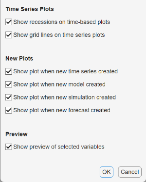
All environment preferences are on by default.
Econometric Modeler does not apply plot preference adjustments retroactively; plot adjustments persist to future Econometric Modeler sessions.
Import Time Series Variables
The data set can exist in the MATLAB Workspace or in a MAT-file that you can access from your machine.
To import a data set from the Workspace, on the Modeler tab, in the Import section, click
 . In the Import Data dialog box, click
the check box for the variable containing the data, and then click
Import. All variables in the Workspace of the
supported data type appear in the dialog box, but you can choose one
only.
. In the Import Data dialog box, click
the check box for the variable containing the data, and then click
Import. All variables in the Workspace of the
supported data type appear in the dialog box, but you can choose one
only.To import data from a MAT-file, in the Import section, click the drop-down menu under Import, then select
Import From MAT-file. In the Select MAT-file dialog box, browse to the folder containing the data set, then double-click the MAT-file.
After you import data, Econometric Modeler performs all the following actions.
The name of each variable (column) in the data set appears in the Time Series pane.
The value of the variable selected in the Time Series pane appears in the Preview pane. To display or operate on a different variable, select it.
A time series plot including all variables appears in the Plot(
VariableName) figure window, whereVariableNameis the name of one of the variables in the Time Series pane.
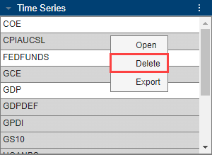
You can interact with the variables in the Time Series pane in several ways.
To select a variable to perform a statistical test or create a plot, for example, click the variable in the Time Series pane. If you double-click the variable instead, then the app also plots it in a separate time series plot.
To open, delete, or export a variable, right-click it in the Time Series pane. Then, from the context menu, choose the desired action.
To select or operate on multiple time series simultaneously, press Ctrl and click each variable you want to use.
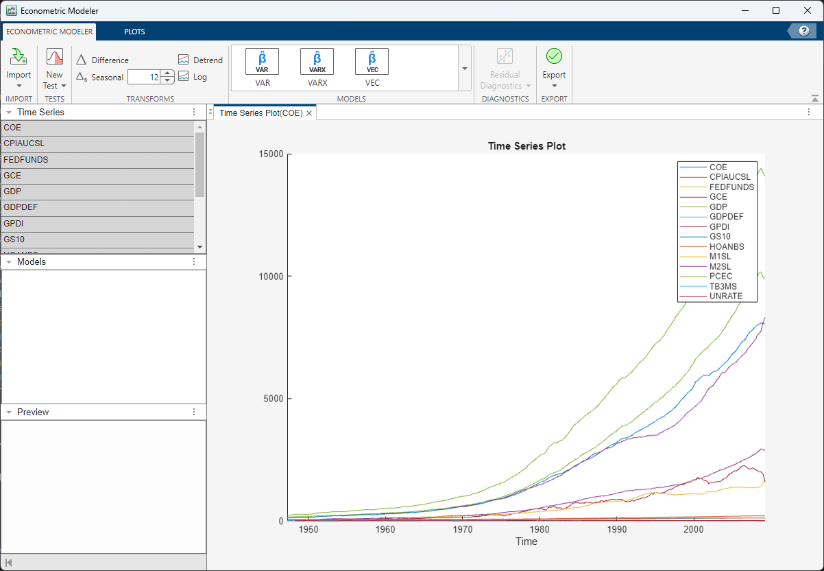
Consider importing the data in the Data_USEconModel MAT-file.
At the command line, load the data into the Workspace.
load Data_USEconModelIn Econometric Modeler, in the Import section of the Modeler tab, click
. The Import Data dialog box
appears.Data_USEconModelstores several variables. Data, DataTable, and DataTimeTable contain the same data, but DataTable is a table, and DataTimeTable is a timetable. Import DataTimeTable by selecting the corresponding check box, then clicking Import.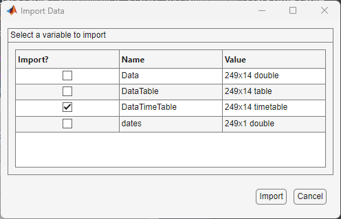
All variables in DataTimeTable appear in the
Time Series pane. Suppose that you want to retain
COE, FEDFUNDS, and
GDP only. Select all other variables, right-click one
of them, and select Delete.
After working in the app, you can import another data set. After you click Import, Econometric Modeler displays the following dialog box.
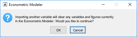
If you click Yes, Econometric Modeler deletes all variables from the Time Series and Models panes, and then it closes all documents in the right pane.
Perform Exploratory Data Analysis
An exploratory data analysis starts with characterizing your time series and measuring the relationships among them. This exploration includes determining whether the series that grow exponentially, contain trends, or are nonstationary, and then transform them appropriately. If your goals include business cycle analysis, you can apply a data filter to the series to decompose it into trend and cyclical components. Regardless, an exploratory analysis usually includes iterating among visualizing the data, performing statistical specification and model identification tests, and transforming the data.
If you plan to form a predictive model, your exploration should include determining the structural features of the model.
To build an ARIMA model for your transformed series, identify the model form by applying Box-Jenkins methodology [1], which includes finding significant lags from the serial correlation structure of the response series.
To build a conditional variance model (for example, GARCH), assess whether the series contain volatility clustering and significant lags.
To build a multiple regression model, identify collinear predictors and those predictors that are linearly related to the response.
For multivariate models, in addition to univariate analyses, you can test whether series are cointegrated.
Visualizing Time Series Data
After you import a data set, Econometric Modeler selects all variables in the
imported data and displays a time series plot of them in the right pane by
default. For example, after you import DataTimeTable
in the Data_USEconModel data set, the app displays this time
series plot.
To create your own time series plot:
In the Time Series pane, select the series for the plot.
Click the Plots tab in the toolstrip.
Click the button for the type of plot.
Econometric Modeler supports the following time series plots.
| Plot | Goals |
|---|---|
Time series ( |
|
Autocorrelation function
( |
|
Partial ACF ( |
|
Correlations ( |
|
You can interact with a plot by:
Right-clicking the plot and choosing the action in the menu
Expanding the axes toolbar at the top right side of the figure
 and selecting an action
Using plot-specific options and parameters on the plot tab
Supported interactions vary by plot type.
Save a figure — Right-click the figure, then select Export. Save the figure that appears.
Add or remove time series in a plot — Right-click the figure, point to Show Time Series menu, then select the time series to add or remove.
Toggle recession bands for time-stamped data — Right-click a time series plot, then select Show Recessions or expand the axes toolbar
, then click
 . For details on recession bands,
see
. For details on recession bands,
see recessionplot.Show grid lines — Expand the axes toolbar
, then click
 .
.Toggle legend — Expand the axes toolbar
, then click
 .
.Pan — Expand the axes toolbar
, then click
 . For more details on panning, see
Explore Data.
. For more details on panning, see
Explore Data.Zoom — Expand the axes toolbar
. To zoom in, click
 . To zoom out, click
 . For more details, see Explore Data.
Restore view — To return the plot to its original view after you pan or zoom, expand the axes toolbar
, then click
 .
.
For serial correlation function plots, additional options exist in the ACF or PACF tabs. You can specify the:
Number of lags to display
Number of standard deviations for the confidence bands
MA or AR order in which the theoretical ACF or PACF, respectively, is effectively zero
Econometric Modeler updates the plot in real time as you adjust the parameters.
As you explore your data, plots and computation results accumulate in the right pane under tabs. You can customize the display of the documents in the right pane to, for example, view multiple plots simultaneously, by performing any of the following actions:
Orient the plot tabs by dragging them into different sections of the right pane. As you drag a plot, the app highlights possible sections in which to place it. To undo the last document or figure window positioning, pause on the dot located in the middle of the partition, then click
 when it appears.
Click the Document Actions button
 on the upper-right corner of the
document. Options include:
on the upper-right corner of the
document. Options include:Tile All — Choose a layout for multiple plots.
Tab Position — Select where to display the figure tab.
Consider an ARIMA model for the effective federal funds rate
(FEDFUNDS). To identify the model characteristics (for
example, the number of AR or MA lags), plot the time series, ACF, and PACF side-by-side.
In the Time Series pane, double-click
FEDFUNDS.On the Plots tab, click ACF.
On the Plots tab, click PACF.
Click the Plot(FEDFUNDS) figure window and drag it to the left side of the right pane. Click the PACF(FEDFUNDS) figure window and drag it to the bottom right of the pane.
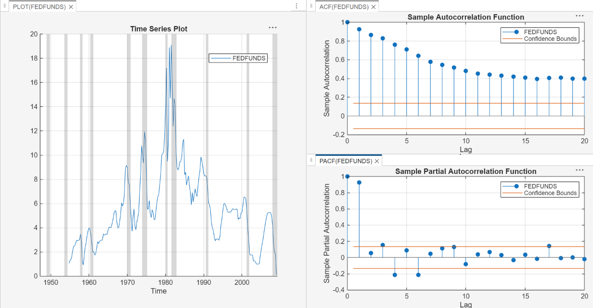
The ACF dies out slowly and the PACF cuts off after the first lag. The behavior of the ACF suggests that the time series must be transformed before you choose on the form of the ARIMA model.
In the right pane, observe the dot in the middle of the horizontal partition
between the correlograms (below the Lag
x axis label of the ACF). To undo this correlogram
positioning, that is, separate the correlograms by tabs, pause on the dot and
click ![]() when it appears.
when it appears.
Performing Specification and Model Identification Hypothesis Tests
You can perform hypothesis tests to confirm time series properties that you obtain visually or test for properties that are difficult to see. Econometric Modeler enables you to run tests multiple times with parameter settings.
Econometric Modeler supports these tests for univariate series.
| Test | Hypotheses |
|---|---|
Augmented Dickey-Fuller
| H0: Series has a unit root. H1: Series is stationary. For details on the
supported parameters, see |
Kwiatkowski, Phillips, Schmidt, Shin (KPSS)
| H0: Series is trend stationary. H1: Series has a unit root. For details on the
supported parameters, see |
Leybourne-McCabe | H0: Series is a trend stationary AR(p) process. H1: Series is an ARIMA(p,1,1) process. To specify p,
adjust the Number of Lags
parameter. For details on the supported parameters, see
|
Phillips-Peron | H0: Series has a unit root. H1: Series is stationary. For details on the
supported parameters, see |
Variance ratio | H0: Series is a random walk. H1: Series is not a random walk. For details on
the supported parameters, see |
Engle's ARCH | H0: Series exhibits no conditional heteroscedasticity (ARCH effects). H1: Series is an ARCH(p) model, with p > 0. To specify
p, adjust the Number of
Lags parameter. For details on the
supported parameters, see |
Ljung-Box Q-test | H0: Series exhibits no autocorrelation in the first m lags, that is, corresponding coefficients are jointly zero. H1: Series has at least one nonzero autocorrelation coefficient ρj, j ∈ {1,…,m}. To specify
m, adjust the Number of
Lags parameter. For details on the
supported parameters, see |
Note
Before conducting tests, Econometric Modeler removes leading and
trailing missing values (NaN values) in the series.
Engle's ARCH test does not support missing values within the series,
that is, NaN values preceded and succeeded by
observations.
The stationarity test results suggest whether you should transform a series to stabilize it, and which transformation is appropriate. For ARIMA models, stationarity test results suggest whether to include degrees of integration. Engle's ARCH test results indicate whether the series exhibits volatility clustering and suggests lags to include in a GARCH model. Ljung-Box Q-test results suggest how many AR lags are required in an ARIMA model.
To perform a univariate test on a time series in Econometric Modeler:
Select the time series variable in the Time Series pane.
On the Modeler tab, in the Tests section, click Add Test.
In the test gallery, click the test you want to conduct. A new tab for the test type appears in the toolstrip, and a new document for the test results appears in the right pane.
On the test type tab, in the Settings section, adjust the settings for the test. For example, consider performing an Engle's ARCH test. On the ARCH tab, in the Settings section, select the number of lags in the test statistic using the Number of Lags spin box, or the significance level (that is, the value of α) using the Significance Level spin box.
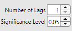
On the test-type tab, in the Tests section, click Run Test. The test results, including whether to reject the null hypothesis, the p-value, and the parameter settings, appear in a new row in the Results table of the test results document. The app highlights tests that reject the null hypothesis in red and tests that retain the null hypothesis in green.
If you run multiple tests on a particular series, the results of each test appear as a new row in the Results table. To remove a row from the Results table, select the corresponding check box in the Select column, then click Clear Tests in the test-type tab.
Note
Multiple testing inflates the false discovery rate. One conservative way to maintain an overall false discovery rate of α is to apply the Bonferroni correction to the significance level of each test. That is, for a total of t tests, set Significance Level value to α/t.
Econometric Modeler supports these tests and diagnostics for multiple series.
| Tests and Diagnostics | Description |
|---|---|
Belsley Collinearity Diagnostics
| For details on the supported parameters and
results, see |
Engle-Granger | H0: The series do not exhibit cointegration. H1: The series exhibit cointegration. For
details on the supported parameters, see |
Johansen | For a specified cointegration rank r:
For details on the supported parameters,
see |
To diagnose multiple series in Econometric Modeler:
Select at least two variables in the Time Series pane.
On the Modeler tab, in the Tests section, click Add Test.
In the tests gallery, select the diagnostics you want to run. A new tab for the diagnostic appears in the toolstrip, and a new document for the results appears in the right pane.
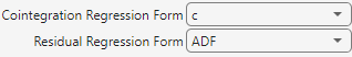
On the tab for the diagnostic, you can adjust parameters for the diagnostic in the appropriate section. For example, consider conducting an Engle-Granger cointegration test on the selected series. In the tests gallery, select Engle-Granger Test. On the EGCI tab, in the Settings section, select the cointegration regression form by using the Cointegration Regression Form list and select the test to conduct on the regression residuals by using the Residual Regression Form list.
For example, consider a predictive model containing Canadian
inflation and interest rates as predictor variables. Determine whether the
variables are collinear. The Data_Canada data set contains
the time series.
Import the
DataTimeTablevariable in theData_Canadadata set into Econometric Modeler (see Import Time Series Variables). The time series plot appears in the right pane.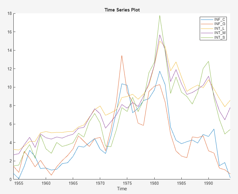
All series appear to contain autocorrelation. Although you should remove autocorrelation from predictor variables before creating a predictive model, this example proceeds without removing autocorrelation.
In the Tests section, click Add Test. In the Collinearity section, click Belsley Collinearity Diagnostics.
Econometric Modeler creates a new tab for the Belsley collinearity diagnostics in the toolstrip, and it creates a new document for the results in the right pane. The results contains a table of the singular values, condition indices, and the variance-decomposition proportions for each series. Rows Econometric Modeler highlights in yellow have a condition index greater than the tolerance specified by the Condition Index parameter value (default is
30) in the Tolerances section of the Collin tab. The columns of the table labeled with series names form the matrix of variance-decomposition proportions. Those series with variance-decomposition proportion greater than the tolerance specified by the Variance-Decomposition Proportion parameter value (default is0.5) in the highlighted row exhibit multicollinearity.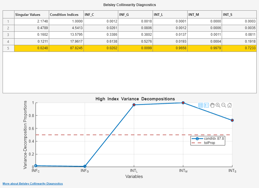
Because their variance-decomposition proportions are above the tolerance (default tolerance is
0.5) for the condition index, the collinear predictors areINT_L,INT_M, andINT_S.You can add or remove time series from the diagnostics. For example, remove the inflation rates from the diagnostics by performing the following procedure.
In the test-results document, right-click the Results table or plot.
Point to Show Time Series. A list of all variables appears.
Remove the inflation rate series
INF_CandINF_Gfrom the diagnostics by deselecting the corresponding check boxes. As you deselect series, Econometric Modeler recomputes the results based on the selected series.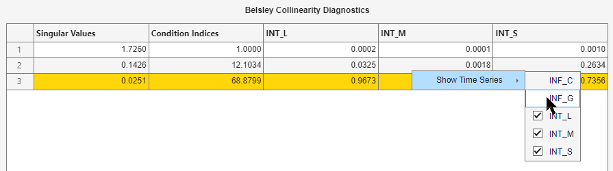
For more details on the Belsley collinearity diagnostics results and
multicollinearity, see collintest and Time Series Regression II: Collinearity and Estimator Variance.
Transforming Time Series
The Box-Jenkins methodology [1] for ARIMA model selection assumes that the response series is stationary, and spurious regression models can result from a model containing nonstationary predictors and response variables (for more details, see Time Series Regression IV: Spurious Regression). To stabilize your series, Econometric Modeler supports these transformations in the Transforms section of the Modeler tab.
| Transformation | Use When Series ... | Notes |
|---|---|---|
Log | Has an exponential trend or variance that grows with its levels | All values in the series must be positive. |
Linear detrend | Has a linear deterministic trend that can be identified using least squares | When Econometric Modeler detrends the series, it
ignores leading or trailing missing
( If any
missing values occur between observed values, then the
app returns a vector of |
First-order difference | Has a stochastic trend | Econometric Modeler prepends the differenced series with
a NaN value. This action ensures that the
differenced series has the same length and time base as the
original series. |
Seasonal difference | Has a seasonal, stochastic trend | You can specify the period in a season using the
spin box. For example, Econometric
Modeler prepends the differenced series with
|
For more details, see Data Transformations.
To transform a variable, select the variable in the Time Series pane, then click a transformation. After you transform a series, a new variable representing the transformed series appears in the Time Series pane. Also, Econometric Modeler plots and selects the new variable. To create the variable name, the app appends the transformation name to the end of the variable name. You can rename the transformed variable by clicking it twice in the Time Series to select the text of the variable name, and then entering the new name. You can select multiple series by pressing Ctrl and clicking each series, and then apply the same transformation to the selected series simultaneously. The app creates new variables for each series, appends the transformation name to the end of each transformed variable name, and plots the transformed variables in the same figure.
For example, suppose that the GDP series in
Data_USEconModel has an exponential trend and a
stochastic trend. Stabilize the GDP by applying the log transformation and then
applying the second difference.
Import the
DataTimeTablevariable in theData_USEconModeldata set into the Econometric Modeler (see Import Time Series Variables).In the Time Series pane, select
GDP.On the Modeler tab, in the Transforms section, click Log. The app creates a variable named
GDP_Log, which appears in the Time Series pane, and displays a plot for the time series.In the Transforms section, click Difference. The app creates a variable named
GDP_Log_Diffand displays a plot for the time series.In the Transforms section, click Difference. The app creates a variable called
GDP_Log_Diff_Diffand displays a plot for the time series.
GDP_Log_Diff_Diff is the stabilized
GDP.
Decomposing Time Series
The Econometric
Modeler app enables you to decompose economic time series into the
long- and short-term components by applying several data filters. To decompose
time series variables, choose at least one time series in the Time
Series pane, then, on the Modeler tab, in
the Filters section, click the Filter
Data button ![]() . In the
. In the Business Cycle
Filters menu, choose a data filter. In the
Type Filter dialog, adjust the associated
parameters, which apply to all selected time series, and then click
Filter.
| Data Filter | Parameters |
|---|---|
| Hodrick-Prescott Filter |
For more details, see |
| Baxter-King Filter |
For more details, see |
| Christiano-Fitzgerald Filter |
For more details, see |
| Hamilton Filter |
For more details, see |
After you decompose the time series, Economic Modeler plots each component in
the same figure, but on separate axes (the cycle on the left
y axis and the trend on the right y
axis). The app returns the components as variables in the Time
Series pane; the variable name follows the pattern
filteredSeries_filterType_component,
where filteredSeries is
the time series being filtered,
filterType is the
abbreviated data filter, and
component is either
Cycle or Trend.
You can treat the returned cycle and trend components like any other time series variable, for example, you can select them in the Time Series pane and plot them, conduct hypothesis tests on them, model them, and forecast models of them.
For example, consider decomposing the US post-WWII, seasonally adjusted, quarterly, real gross national product (GNP) by applying the Hodrick-Prescott filter.
Import the
DataTimeTablevariable in theData_GNPdata set into the Econometric Modeler (see Import Time Series Variables).On the Modeler tab, in the Time Series pane, select
GNPR.In the Filters section, click Filter Data > Hodrick-Prescott Filter. The Hodrick-Prescott Filter dialog containing the associated parameter settings and a plot of the time series and long-term trend component, for the parameter settings, appears.
The series has a quarterly periodicity. Therefore, a smoothing parameter value of 1600 applies. In the Hodrick-Prescott Filter dialog, accept the default parameter values and click Filter to apply the two-sided Hodrick-Prescott filter to the series.
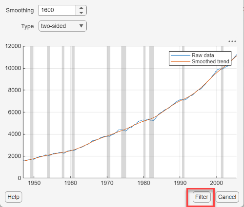
On the Modeler tab, a time series plot appears in the right pane showing the cyclical component (right y axis) and trend component (left y axis).
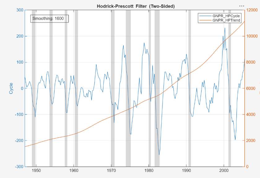
In the Time Series pane, the variable
GNPR_HPCycleis the cyclical component andGNPR_HPTrendis the trend component.In the Time Series pane, double-click
GNPR_HPCycle. A plot of only the cyclical component appears in the right pane.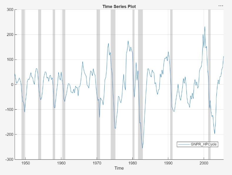
Real GNP falls sharply just before and during periods of recession.
Fit Models to Data
The results of an exploratory data analysis can suggest several candidate models. To choose a model, in the Time Series pane, select the time series for the response. On the Modeler tab, in the Models section, click a model or click one in the models gallery. Econometric Modeler allows you to select only those models that are appropriate for the number of the selected response series. After you select a model, you configure it for estimation.
Econometric Modeler supports the following models.
| Model | Response | Type |
|---|---|---|
| Conditional mean: ARIMA Models section | Univariate | Stationary autoregressive (AR)
For details,
see What Are Autoregressive (AR) Models?, |
| Univariate | Stationary moving average (MA)
For details,
see What Are Moving Average (MA) Models?, | |
| Univariate | Stationary ARMA For details,
see What Are Autoregressive Moving Average (ARMA) Models?, | |
| Univariate | Nonstationary, integrated ARMA (ARIMA)
For details,
see What Are Autoregressive Integrated Moving Average (ARIMA) Models?, | |
| Univariate | Seasonal (Multiplicative) ARIMA (SARIMA)
For details,
see What Are Seasonal ARIMA (SARIMA) Models?, | |
| Univariate | ARIMA including exogenous predictors (ARIMAX)
For details,
see What Are ARIMAX Models?, | |
| Univariate | Seasonal ARIMAX | |
| Conditional variance: GARCH Models section | Univariate | Generalized autoregressive conditional heteroscedastic
(GARCH) For details,
see GARCH Model, |
| Univariate | Exponential GARCH (EGARCH) For details,
see EGARCH Model, | |
| Univariate | Glosten, Jagannathan, and Runkle (GJR)
| |
| Multiple linear regression: Regression Models section | Univariate | Multiple linear regression For details,
see Time Series Regression I: Linear Models, |
| Univariate | Regression model with ARMA errors
For details,
see What Are Regression Models with Time Series Errors, | |
| Vector Autoregression Models: Multivariate Models section | Multivariate | Stationary vector autoregression (VAR)
For details,
see Vector Autoregression (VAR) Models and |
| Multivariate | VAR including exogenous variable (VARX)
For details,
see Vector Autoregression (VAR) Models and | |
| Multivariate | Vector error-correction (VEC) or
cointegrated VAR
For details,
see |
For univariate conditional mean model estimation, SARIMA and SARIMAX are the most flexible models. You can create any conditional mean model that excludes exogenous predictors by clicking SARIMA, or you can create any conditional mean model that includes at least one exogenous predictor by clicking SARIMAX.
For multivariate model estimation, the model you choose depends on whether the selected time series are stationary or cointegrated. For stationary series, create a VAR model by clicking VAR. To include exogenous predictors, click VARX instead. For cointegrated series, click VEC.
After you select a model, the app displays the Type
Model Parameters dialog box, where Type is the model
type. For example, this figure shows the SARIMAX Model Parameters dialog box.
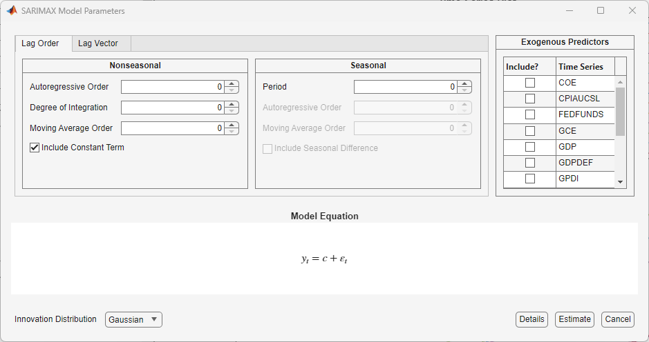
Adjustable parameters in the Type Model Parameters
window depend on Type; Econometric Modeler
sets default values regardless of the characteristics of the time series and
periodicity of the data. In general, adjustable parameters include:
Deterministic terms and linear regression coefficients corresponding to predictor variables (see Adjusting Deterministic Terms and Regression Component Parameters)
Time series component parameters for univariate models, which include seasonal and nonseasonal lags and degrees of integration (see Adjusting Time Series Component Parameters for Univariate Models)
Time series component parameters for multivariate models, which include AR lags and AR coefficient elements to specify equality constraints during estimation (see Adjusting Time Series Component Parameters for Multivariate Models)
For univariate models, the innovation distribution (see Adjusting Innovation Distribution Parameters for Univariate Models)
As you adjust parameter values, the equation in the Model Equation section changes to match your specifications. Adjustable parameters correspond to input and name-value pair arguments described in corresponding model creation reference pages. For details, see the function reference page for a specific model. Regardless of the model you choose, all unspecified coefficients in the model are unknown and estimable, including the t-distribution degrees of freedom parameter (when you specify a t innovation distribution).
Note
Econometric Modeler does not support:
Optimization option adjustments for estimation.
Composite conditional mean and variance models. For details, see Specify Conditional Mean and Variance Models.
Equality constraints on univariate model parameters during estimation (except for holding some parameters fixed at zero during estimation).
To adjust optimization options, estimate composite conditional mean and variance models, or apply equality constraints, use the MATLAB command line.
Adjusting Deterministic Terms and Regression Component Parameters
Supported deterministic terms depend on the selected model and include a model
constant (offset or intercept) and linear time trend. To include a model
constant (offset or intercept) term, select the Include Constant
Term or Include Offset check box. Similar
for a linear time trend, select the Include Trend check
box. To remove a deterministic term (that is, constrain it to zero during
estimation), clear the check box. The location and type of the check box in the
Type Model Parameters dialog box depends on the
model type. By default, Econometric Modeler includes a model constant in all
model types except conditional variance models.
To select predictors for the regression component, in the Exogenous Predictors list, select the check box in the Include column corresponding to the predictors you want to include in the model. By default, the app does not include a regression component in any model type.
If you select ARIMAX, SARIMAX, RegARMA, or VARX, you must choose at least one predictor.
If you select MLR, you can specify one of the following:
An MLR model when you choose at least one predictor
A constant mean model (intercept-only model) when you clear all check boxes in the Include column and select the Include Intercept check box
An error-only model when you clear all check boxes in the Include column and clear the Include Intercept check box
Consider a linear regression model of GDP onto CPI and the unemployment rate. To specify the regression:
Import the
DataTimeTablevariable in theData_USEconModeldata set into the Econometric Modeler (see Import Time Series Variables).In the Time Series pane, select the response variable
GDP.On the Modeler tab, in the Models section, click the arrow to display the models gallery.
In the models gallery, in the Regression Models section, click MLR.
In the MLR Model Parameters dialog box, in the Include column, select the CPIAUCSL and UNRATE check boxes.
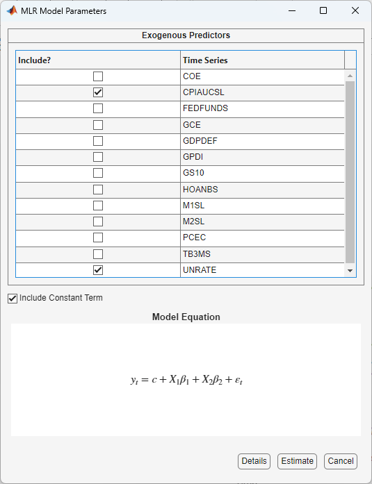
Click the Estimate button.
Adjusting Time Series Component Parameters for Univariate Models
In general for univariate models, time series component parameters contain lags to include in the seasonal and nonseasonal lag operator polynomials, and seasonal and nonseasonal degrees of integration.
For conditional mean models, you can specify seasonal and nonseasonal autoregressive lags, and seasonal and nonseasonal moving average lags. Also, you can specify up to 2 nonseasonal degrees of integration and up to 1 seasonal degrees of integration.
For conditional variance models, you can specify ARCH and GARCH lags. EGARCH and GJR models also support leverage lags.
For regression models with ARMA errors, you can specify nonseasonal autoregressive and moving average lags. For models containing seasonal lags or degrees of seasonal or nonseasonal integration, use the command line instead.
Econometric Modeler supports two options to adjust the
parameters. The adjustment options are on separate tabs of the
Type Model Parameters dialog box: the
Lag Order and Lag Vector tabs. On
the Lag Order tab, you can specify the
orders of lag operator polynomials. This feature
enables you to include all lags efficiently, from 1 through the specified order,
in a lag operator polynomial. On the Lag Vector tab, you
can specify the individual lags that comprise a lag
operator polynomial. This feature is well suited for creating flexible models.
For more details, see Specifying Univariate Lag Operator Polynomials Interactively.
Adjusting Innovation Distribution Parameters for Univariate Models
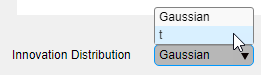
For univariate models, you can specify that the distribution of the innovations is Gaussian. For all models, except multiple linear regression models, you can specify the Student's t instead to address leptokurtic innovation distributions (for more details, see Maximum Likelihood Estimation for Conditional Mean Models, Maximum Likelihood Estimation for Conditional Variance Models, or Maximum Likelihood Estimation of regARIMA Models). If you specify the t distribution, then Econometric Modeler estimates its degrees of freedom parameter using maximum likelihood.
By default, Econometric Modeler uses the Gaussian distribution for the
innovations. To change the innovation distribution, in the
Type Model Parameters dialog box, from the
Innovation Distribution button, select a distribution
in the list.
Adjusting Time Series Component Parameters for Multivariate Models
Supported time series component parameters for multivariate models depend on the model type. All types enable you to include nonseasonal AR lag coefficients. However, VEC models additionally support the following parameters specifications:
The Johansen model form, which specifies which deterministic terms (overall or within the cointegrating relation) to include in the model. For details, see Johansen Form.
Cointegration rank r
Adjustment speed matrix A
Cointegration matrix B
This figure is an example of the Type Model
Parameters dialog box.
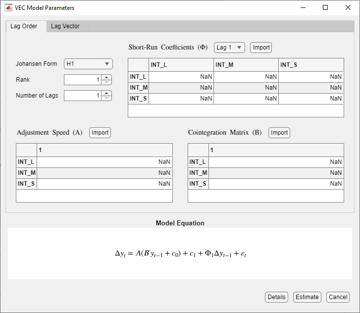
Like univariate models, Econometric Modeler supports adjusting the AR or short-run lag operator polynomial efficiently by specifying the lag order (Lag Order tab) or, for flexibility, by specifying individual lags (Lag Vector tab). Unlike univariate models, Econometric Modeler supports estimation equality constraints on individual entries of the AR or short-run lag coefficient matrix, which correspond to self- or cross-variable lag coefficients in the model. Coefficient constraints enable you to test economic scenarios. Econometric Modeler holds the specified values fixed during estimation.
For VEC models, you can specify equality constraints on the entire matrix
A or B, except for Johansen forms
H* and H1* which support equality
constraints only for A.
To specify such equality constraints:
In the
TypeModel Parameters dialog box, select the lag to constrain by using the AR Coefficients (ϕ) (VAR or VARX) or Short-Run Coefficients (Φ) (for VEC) list.Perform either one of the following alternatives:
Click the elements of the matrices to constrain, and then enter the value. Econometric Modeler estimates all
NaNentries.Import a matrix.
At the command line, create an appropriately sized matrix of constraints or mix of constraints and
NaNvalues for AR or short-run lags.In Econometric Modeler, in the
TypeModel Parameters dialog box, click Import.In the dialog box, select the variable to import for the coefficient matrix.
For details, see Specifying Multivariate Lag Operator Polynomials and Coefficient Constraints Interactively.
Estimating a Univariate Model
Econometric Modeler treats all parameters in the model as unknown and
estimable. After you specify a model, fit it to the data by clicking
Estimate in the Type Model
Parameters dialog box.
Note
Econometric Modeler requires initial values for estimable parameters and presample observations to initialize the model for estimation. Econometric Modeler always chooses the default initial and presample values as described in the
estimatereference page of the model you want to estimate.If Econometric Modeler issues an error during estimation, then:
The specified model poorly describes the data. Adjust model parameters, then estimate the new model.
At the command line, adjust optimization options and estimate the model. For details, see Optimization Settings for Conditional Mean Model Estimation, Optimization Settings for Conditional Variance Model Estimation, or Optimization Settings for regARIMA Model Estimation.
After you estimate a model:
A new variable that describes the estimated model appears in the Models pane with the name
Type_response.Typeis the model type andresponseis the response variable to which Econometric Modeler fit the model, for example,ARIMA_FEDFUNDS.You operate on an estimated model in the Models pane by right-clicking it. In addition to the options available for time series variables (see Import Time Series Variables), the context menu includes the
Modifyoption, which enables you to modify and re-estimate a model. For example, right-click a model and selectModify. Then, in theTypeModel Parameters dialog box, adjust parameters and click Estimate.The object display of the model appears in the Preview pane.
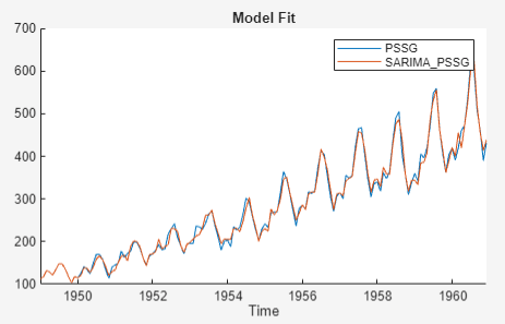
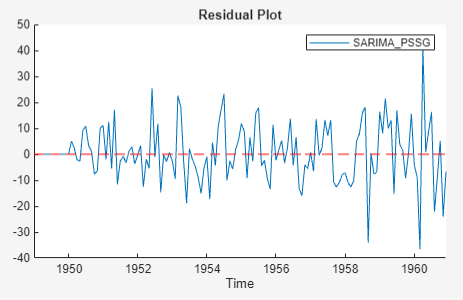
The Fit(
Type_response) document summarizing the estimation results appears in the right pane. The results depend on the model type. For conditional mean and regression models, results include:Model Fit — A time series plot of the response series and the fitted values
Parameters — An estimation summary table containing parameter estimates, standard errors, and t statistics and p-values for testing the null hypothesis that the corresponding parameter is 0
Residual Plot — A time series plot of the residuals
Goodness of Fit — Model fit statistics, such as the AIC.
For conditional variance models, the results also include an estimation summary table and goodness-of-fit statistics, but Econometric Modeler plots the following series instead of the fitted values and residuals:
Conditional Variances — A time series plot of the inferred conditional variances
Standardized Residuals — A time series plot of the standardized residuals , where c is the estimated offset
You can interact with individual plots by expanding the axes toolbar
and selecting an interaction (see
Visualizing Time Series Data).
You can also interact with the summary by right-clicking a plot in
the summary. Options include:Export — Place plot in a separate figure window.
Show Model — Display the summary of another estimated model by pointing to Show Model, then selecting a model in the list.
Show Recessions — Plot recession bands in time series plots.
Consider a SARIMA(0,1,1)×(0,1,1)12 for the monthly
international airline passenger numbers from 1949 to 1960 in the
Data_Airline data set. To estimate this model using the
Econometric Modeler:
Download the
Data_Airline.matMAT-file into your current folder, and then load it into the workspace.fldr = pwd; openExample("Data_Airline.mat",workDir=fldr); load(fullfile(fldr,"Data_Airline.mat"))
To change the folder to which to download the data set, set
fldrto its absolute path.Import the
DataTimeTablevariable in theData_Airlinedata set into Econometric Modeler (see Import Time Series Variables).On the Modeler tab, in the Models section, click the arrow > SARIMA.
In the SARIMA Model Parameters dialog box, on the Lag Order tab:
Nonseasonal section
Set Autoregressive Order (p) to
0.Clear the Include Constant Term check box.
Seasonal section
Set Autoregressive Order (ps) to
0.The Seasonality (s) parameter is
12by default; this setting indicates monthly periodicity.
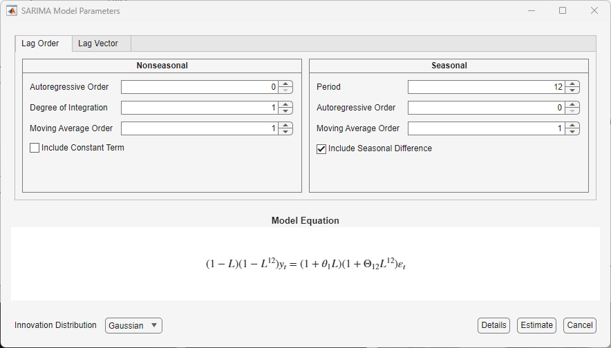
Click Estimate.
As a result:
A variable named
SARIMA_PSSGappears in the Models pane.The value of
SARIMA_PSSGappears in the Preview pane.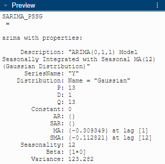
An estimation summary appears in the new Fit(SARIMA_PSSG) document.
Estimating a Multivariate Model
Econometric Modeler treats all parameters in the model as unknown and estimable by default. However, unlike univariate models, Econometric Modeler supports equality constraints on some parameters for estimation. You can specify coefficient values in the app or import a lag coefficient matrix from the workspace.
After you configure the model, fit it to the data by clicking
Estimate in the Type Model
Parameters dialog box.
Note
To initialize the model for estimation, Econometric Modeler removes the first p observations from the response data to use as a presample, and then the function fits the model to the remaining observations.
If Econometric Modeler issues an error during estimation, the specified model poorly describes the data. Adjust model parameters, and then estimate the new model.
After you estimate a model, Econometric Modeler shows results similar to that of univariate estimation (see Estimating a Univariate Model), and you can interact with an estimated multivariate model in the same ways as with univariate models. Notable differences include:
A new variable that describes the estimated model appears in the Models pane with the name
Typej, whereTypeis the model type andjis estimated model j of that type, for example,VAR2is the second estimated VAR model during the session.The Fit(
Type_response) document summarizing the estimation results appears in the right pane. However, the plots shown depend on the model type and the selected time series in the Time Series list at the top of the document. For VAR models, results include:Model Fit — A time series plot of the selected time series and the corresponding fitted values
Residual Plot — A time series plot of the residuals corresponding to the selected time series
For VEC models, the results additionally include a time series plot of the cointegrating relation, which is invariant to the selected time series.
Consider a 3-D VAR(4) model of quarterly measurements of the US gross domestic
product (GDP), M1 money supply, and the 3-month T-bill rate from 1947 through
2009. The file Data_USEconModel.mat contains the series,
among other economic measurements.
To estimate this model using the Econometric Modeler:
Import the
DataTimeTablevariable in theData_USEconModeldata set into Econometric Modeler (see Import Time Series Variables).On the Modeler tab, in the Time Series pane, click
GDP, and then press Ctrl and clickM1SL.Because
GDPandM1SLexhibit exponential growth, use their growth rates in the model. On the Modeler tab, in the Transforms section, click Log, and then click Difference. Change the name of the transformed variables toGDPRateandM1SLRate, respectively.In the Time Series pane, click
TB3MS, and then stabilize the series by clicking, in the Transforms section, Difference. Change the name of the transformed series toTB3MSRate.With
TB3MSRateselected, select the three rate series for the VAR model by pressing Ctrl and clickingGDPRateandM1SLRate.On the Modeler tab, in the Models section, click VAR.
In the VAR Model Parameters dialog box, on the Lag Order tab, set Autoregressive Order (p) to
4.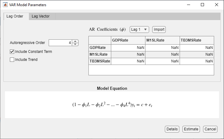
Click Estimate.
As a result:
A variable named
VARappears in the Models pane.The value of
VARappears in the Preview pane.
An estimation summary appears in the new Fit(VAR) document. The plots are relative to the GDPRate series. The indices of the parameter estimates in the Parameters section correspond to the order of the series in the Time Series list (for example
AR{1}(2,3)is the lag 1 AR coefficient of theTB3MSRateseries in the equation of theM1SLRateseries.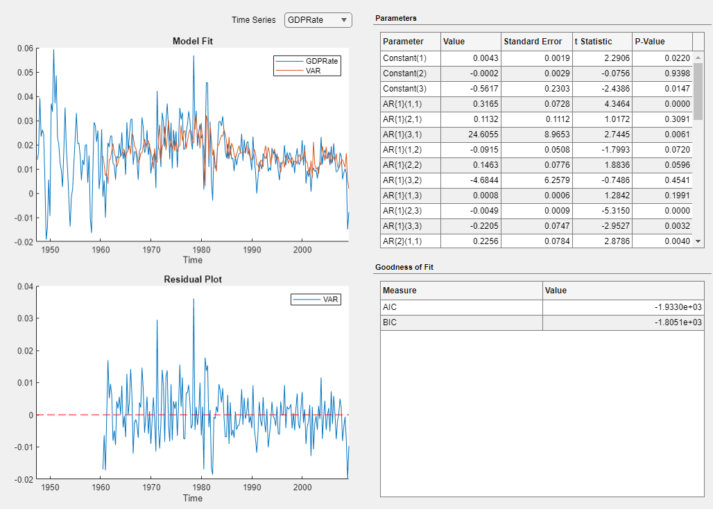
Conduct Goodness-of-Fit Checks
After you estimate a model, a good practice is to determine the adequacy of the fitted model (see Goodness of Fit). Econometric Modeler is well suited for assessing the in-sample fit of a model to data:
Visually determine how well the fitted responses and the response series track each other (for all models except conditional variance models).
Inspect the Lack-of-Fit F-test statistic and p-value.
Perform residual diagnostics.
Visually compare response paths simulated from the model and the response series.
The Lack-of-Fit F test and residual diagnostics help you evaluate model assumptions and determine whether you must respecify the model to address other properties of the data. The Lack-of-Fit F test checks whether the specified model (alternative hypothesis) is a better fit to the data, in terms of explaining variability, than a mean-only model (null hypothesis). If the test statistic or p-value suggest that the mean-only model hypothesis should not be rejected, the specified model must be reconsidered. Residual diagnostics assess model assumptions, including whether the residuals have a mean of zero, and are normally distributed, homoscedastic, and serially uncorrelated. If the residuals do not demonstrate all these properties, then you must determine the severity of the departure, whether to transform the data, and whether to specify a different model. For more details on residual diagnostics, see Time Series Regression VI: Residual Diagnostics and Residual Diagnostics.
To perform goodness-of-fit checks using Econometric Modeler, in the Models pane, select an estimated model. Then, complete the following steps:
Visually assess the in-sample fit for all models (except conditional variance models) by inspecting the Model Fit plot in the Fit document. For multivariate models, Econometric Modeler displays fitted values of one series. You can select a different series in the model to plot by clicking the series in the Time Series list.
Determine whether the model fits to the data significantly better than a mean-only model by inspecting the Lack-of-Fit F-test results. In the Fit(
ModelName) document, in the Goodness of Fit table, in the Measure column, findForProb(F), and compare the corresponding value to a critical value or level of significance. If, for example, the value ofProb(F)is less than a level of significance of 0.05, the specified model fits to the data better than a mean only model.Simulate response paths from the model, and then compare them to the response data. On the Modeler tab, in the Simulate section, click the Simulate button
 . In the Simulate Model Response
dialog, choose the number of simulated paths, select whether to plot the
simulations, and whether to plot summary statistics, and then click the
Simulate button.
. In the Simulate Model Response
dialog, choose the number of simulated paths, select whether to plot the
simulations, and whether to plot summary statistics, and then click the
Simulate button.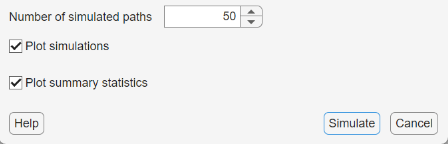
If you choose to plot the simulated paths, a figure with name SIM(
ModelName) appears with the paths and the response data. You can toggle the recession bands, simulated paths, and simulation statistics on or off by right-clicking the figure and selecting the box for the option.Note
Because you cannot operate on simulated values, all actions on the Modeler tab are unavailable, except session export actions in the Export section. To continue working in Econometric Modeler, select a time series in the Time Series pane or a model in the Models pane.
To perform residual diagnostics using Econometric Modeler, in the Models pane, select an estimated model. Then, complete the following steps:
Visually assess whether the residuals are centered on zero, autocorrelated, and heteroscedastic by inspecting, in the Fit(
ModelName) document, the Residual Plot. For multivariate models, Econometric Modeler displays residuals of one series. You can select a different residual series to plot by clicking the corresponding series in the Time Series list.Check additional model assumptions, visually and statistically. On the Modeler tab, in the Diagnostics section, click Model Fit Diagnostics. The diagnostics gallery provides these residual plots and tests.
Alternatively, to view the model estimation summary, plot fitted values or residuals, or conduct tests on residuals of an estimated model:
Select a model in the Models pane.
Click the Plots tab.
In the Plots section, click the arrow and then select one of the plots in the Model Plots section of the gallery.
With a model selected, on the Modeler tab, in the Tests section, click Add Test. Select a test from the Model Residuals section.
Method Diagnostic Model Fit (
Model
                                                Fit
)
View model estimation results Residual Histogram (
ResHist)
Visually assess normality Residual Q-Q Plot (
ResQQ)
Visually assess normality and skewness Residual (
ResACF) Autocorrelation
Visually assess whether residuals are autocorrelated Ljung-Box Q-Test

Test residuals for significant autocorrelation Squared Residuals (
SqResACF) AutocorrelationVisually assess whether residuals have conditional heteroscedasticity Engle's ARCH Test
Test residuals for conditional heteroscedasticity (significant ARCH effects) For multivariate models:
Econometric Modeler plots residual diagnostics for all model series within the same document.
Econometric Modeler runs residual diagnostic tests simultaneously for all series, but it shows results of each residual series separately. You can choose which results to show by clicking, in the test tab, the series in the Time Series list.
Determine whether the residual series is lag-1 autocorrelated, in the Fit(
ModelName) document, in the Goodness of Fit table, in the Measure column, findDurbin-Watson. The corresponding value is the test statistic, it is not a p-value. This table helps you interpret the Durbin-Watson test statistic.Value Description Less than 1Residuals show significant positive lag-1 autocorrelation Between 1and2Residuals show moderate positive lag-1 autocorrelation Close to 2Residuals show no significant lag-1 autocorrelation Between 2and3Residuals show moderate negative lag-1 autocorrelation Greater than 3Residuals show significant negative lag-1 autocorrelation
Note
Another important goodness-of-fit check is predictive-performance assessment. To assess the predictive performance of several models:
Fit a set of models to the data using Econometric Modeler.
Perform residual diagnostics on all models.
Choose a subset of models with desirable residual properties and minimal fit statistics (see Find Model with Best In-Sample Fit).
Export the chosen models to the MATLAB Workspace (see Export Session Results).
Perform a predictive performance assessment at the command line (see Assess Predictive Performance).
For an example, see Compare Predictive Performance After Creating Models Using Econometric Modeler.
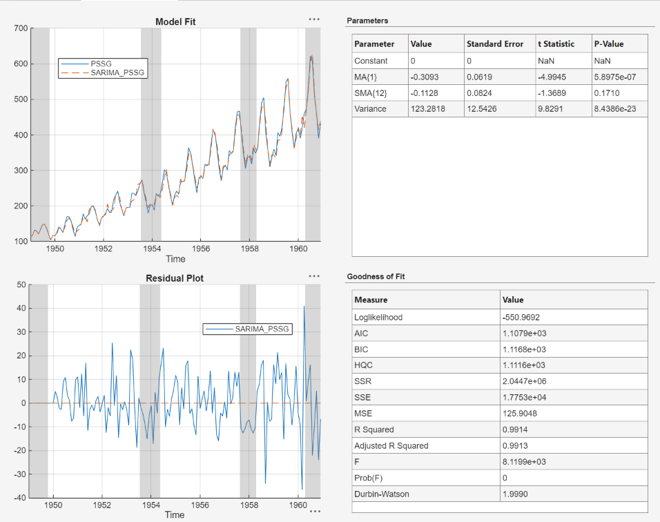
Consider performing goodness-of-fit checks on the estimated SARIMA(0,1,1)×(0,1,1)12 model for the airline counts data in Estimating a Univariate Model.
In the right pane, on the Fit(SARIMA_PSSG) document:
Model Fit suggests that the model fits to the data fairly well.
Residual Plot suggests that the residuals have a mean of zero. However, the residuals appear heteroscedastic and serially correlated.
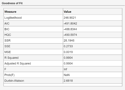
In the Goodness of Fit table, the value of
Prob(F), the p-value of the Lack-of-Fit F test, is0. This result suggests that the specified model fits to the data significantly better than a mean-only model. The value ofDurbin-Watson, the Durbin-Watson test statistic, is1.9990. This result suggests that there's little evidence to conclude that the residuals are lag-1 autocorrelated.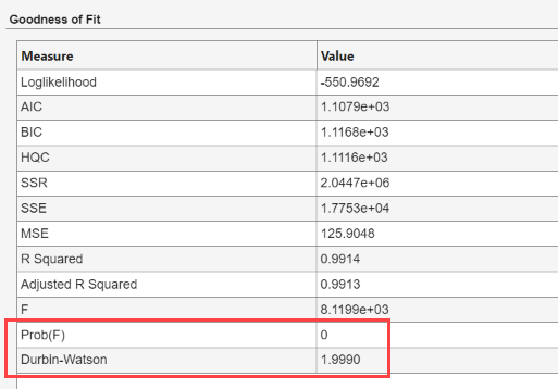
Determine how well the response data matches the model by plotting 50 simulated response paths from the model with the data. On the Modeler tab, in the Simulate section, click Simulate. At the dialog, click Simulate Model Response dialog, click Simulate.
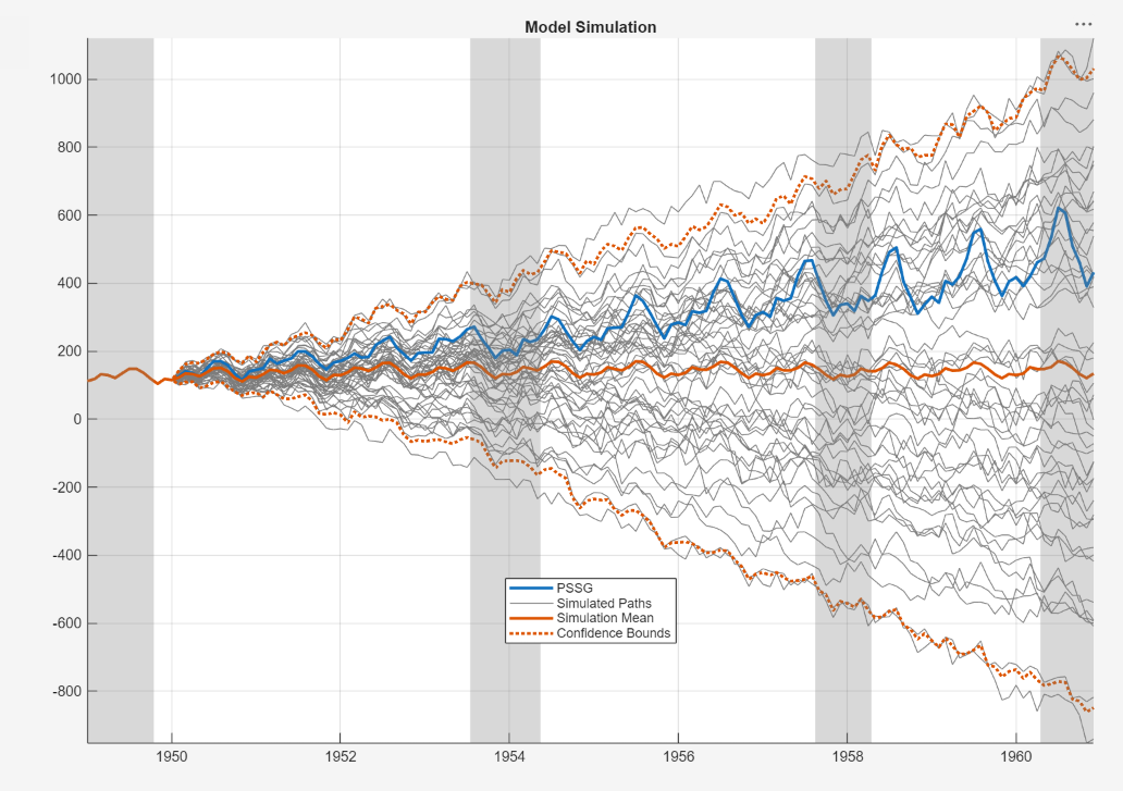
All simulated paths start at period two unless they require a longer presample to initialize the model, which is a common requirement for dynamic models. If a model requires a presample of more than 1 observation, all simulated paths begin at the time point after the end of the presample period. The length of the presample period depends on the dynamic model, see the associated reference page for details. In this case, a SARIMA(0,1,1)×(0,1,1)12 model requires 13 observations; therefore, all simulated paths start at the time period 14 in the in-sample data.
The simulated paths fan out with time, which is characteristic of paths simulated from a nonstationary model. The observed response series is well within the 95% percentile intervals.
On the Modeler tab, in the Diagnostics section, click Model Fit Diagnostics. In the diagnostics gallery:
Click Residual Q-Q Plot. The right pane display a figure window named QQ(SARIMA_PSSG) containing a quantile-quantile plot of the residuals.
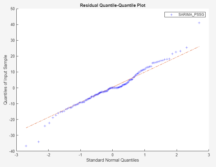
The plot suggests that the residuals are approximately normal, but with slightly heavier tails.
Click Residual Autocorrelation. In the toolstrip, the ACF tab appears and contains plot options. The right pane displays a figure window named ACF(SARIMA_PSSG) containing the ACF of the residuals.
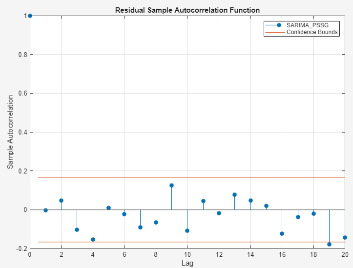
Because almost all the sample autocorrelation values are below the confidence bounds, the residuals are likely not serially correlated. This result is consistent with the Durbin-Watson test statistic.
Click Engle's ARCH Test. On the ARCH tab, in the Tests section, click Run Test to run the test using default options. The right pane displays the ARCH(SARIMA_PSSG) document, which shows the test results in the Results table.
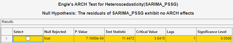
The results suggest rejection of the null hypothesis that the residuals exhibit no ARCH effects at a 5% level of significance. You can try removing heteroscedasticity by applying the log transformation to the series.
Find Model with Best In-Sample Fit
Econometric Modeler enables you to fit multiple related models to a data set efficiently. After you estimate a model, you can estimate other models by iterating the methods in Perform Exploratory Data Analysis, Fit Models to Data, and Conduct Goodness-of-Fit Checks. After each iteration, a new model variable appears in the Models pane.
For models in the same parametric family that you fit to the same response series, you can determine the model with the best parsimonious, in-sample fit among the estimated models by comparing their fit statistics. From a subset of candidate models, to determine the model of best fit using Econometric Modeler:
In the Models pane, double-click an estimated model. In the right pane, estimation results of the model appear in the Fit(
Model) document, whereModelis the name of the selected model.On the Fit(
Model) document, in the Goodness of Fit table, choose a fit statistic and record its value. The available fit statistics areFit Statistic Value Indicating Best Fit Loglikelihood
Greatest Akaike information criterion (AIC)
Least Bayesian information criterion (BIC)
Least Hannan-Quinn Criterion (HQC)
Least Residual sum of squares (SSR)
Least Error sum of squares (SSE)
Least Mean squared error (MSE)
Least R2
Closest to 1 or -1 Adjusted R2
Closest to 1 or -1 Iterate the previous steps for all candidate models.
Choose the model that yields the best fit statistic.
For more details on goodness-of-fit statistics, see Information Criteria for Model Selection.
Consider finding the best-fitting SARIMA model, with a period of 12, for the log
of the airline passenger counts in the Data_Airline data set. Fit
a subset of SARIMA models, considering all combinations of models that include up to
two seasonal and nonseasonal MA lags. Include 1 degree of seasonal and nonseasonal
integration in each model.
Import the
DataTimeTablevariable in theData_Airlinedata set into Econometric Modeler (see Import Time Series Variables).Apply the log transformation to
PSSG(see Transforming Time Series).Fit a SARIMA(0,1,q)×(0,1,q12)12 to
PSSG_Log, where all unknown orders are 0 (see Estimating a Univariate Model).In the right pane, on the Fit(SARIMA_PSSG_Log) document, in the Goodness of Fit table, record the AIC value.
In the Time Series pane, select
PSSG_Log.Iterate steps 4 and 5, but adjust q and q12 to cover the nine permutations of q ∈ {
0,1,2} and q12 ∈ {0,1,2}. Econometric Modeler distinguishes subsequent models of the same type by appending consecutive digits to the end of the variable name.
The resulting AIC values are in this table.
| Model | Variable Name | AIC |
|---|---|---|
| SARIMA(0,1,0)×(0,1,0)12 | SARIMA_PSSG_Log | -491.8042 |
| SARIMA(0,1,0)×(0,1,1)12 | SARIMA_PSSG_Log_2 | -530.5327 |
| SARIMA(0,1,0)×(0,1,2)12 | SARIMA_PSSG_Log_3 | -528.5330 |
| SARIMA(0,1,1)×(0,1,0)12 | SARIMA_PSSG_Log_4 | -508.6853 |
| SARIMA(0,1,1)×(0,1,1)12 | SARIMA_PSSG_Log_5 | -546.3970 |
| SARIMA(0,1,1)×(0,1,2)12 | SARIMA_PSSG_Log_6 | -544.6444 |
| SARIMA(0,1,2)×(0,1,0)12 | SARIMA_PSSG_Log_7 | -506.8027 |
| SARIMA(0,1,2)×(0,1,1)12 | SARIMA_PSSG_Log_8 | -544.4789 |
| SARIMA(0,1,2)×(0,1,2)12 | SARIMA_PSSG_Log_9 | -542.7171 |
Because it yields the minimal AIC, the SARIMA(0,1,1)×(0,1,1)12 model is the model with the best parsimonious, in-sample fit.
Forecast Model with Best In-Sample Fit
Econometric Modeler enables you to forecast responses from an estimated model into a specified forecast horizon. Although you can generate forecasts from any model that does not contain an exogenous regression component, typically, you find the best fitting model first (see Find Model with Best In-Sample Fit), and then generate forecasts from it.
Once you have a model from which to generate forecast, select it from the
Models pane, and then, on the Modeler
tab, in the Forecast section, click
Forecast button ![]() . Forecast options include:
. Forecast options include:
Number of periods in forecast horizon — Positive integer that determines the number of responses to forecast, with respect to the sampling frequency
Method — List of forecasting methods, either
Minimum Mean-Squared Errorfor minimum mean-squared error (MMSE) forecasts and pointwise 95% Wald-based confidence intervals, orSimulationfor simulation-based (Monte Carlo) forecasts and pointwise 95% percentile intervals. For more details, see More About MMSE and Monte Carlo Forecasting.Number of simulated paths — For simulation-based forecasts, positive integer for the number of simulated paths, from which to base the forecasts and confidence intervals
To forecast the model, click Forecast. The right pane
displays a figure window named
FOR(Model) containing the
series, forecasts, and 95% confidence intervals. In the
Forecasts pane, a variable
FOR_, a structure
array, contains the forecasts, and upper and lower confidence bounds.Model
Note
Because you cannot operate on forecasts, all actions on the Modeler tab are unavailable, except session export actions in the Export section. To continue working in Econometric Modeler, select a time series in the Time Series pane or a model in the Models pane.
Consider forecasting the best-fitting SARIMA model fit for the log of the airline
passenger counts in the Data_Airline data set.
Import the
DataTimeTablevariable in theData_Airlinedata set into Econometric Modeler (see Import Time Series Variables).Apply the log transformation to
PSSG(see Transforming Time Series).Fit a SARIMA(0,1,1)×(0,1,1)12 model, the best fitting model, to
PSSGLog.Forecast the estimated model, using MMSE forecasts, into a 3-year (36-month) horizon. With the
SARIMA_PSSG_Logestimated model selected in the Models pane, on the Modeler tab, in the Forecast section, click Forecast. In the Forecast Model Response dialog box, set Number of periods in forecast horizon to36, and then click Forecast.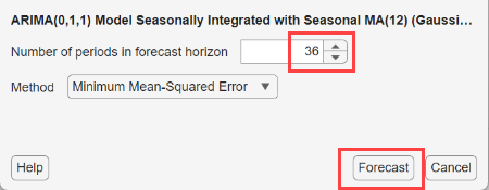
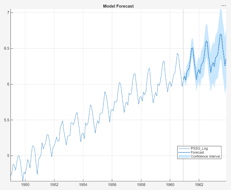
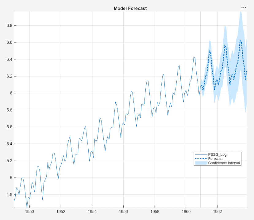
The right pane displays a figure window named FOR(SARIMA_PSSG_Log) containing the series of log airline passenger counts, 3-year monthly MMSE forecasts, and the 95% Wald-based confidence intervals. A vertical line separates the in-sample and forecast periods.
In the Forecasts pane, a variable named FOR_SARIMA_PSSG_Log is a structure array containing the forecasts (
Forecast), the pointwise upper confidence bounds (UpperConfidenceBound), and the lower confidence bounds (LowerConfidenceBound). The Preview pane shows the value of the variable.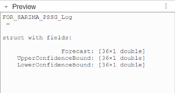
Forecast the estimated model, using Monte Carlo forecasting, into a 3-year (36-month) horizon. Select the
SARIMA_PSSG_Logestimated model selected in the Models pane, on the Modeler tab, in the Forecast section, click Forecast. In the Forecast Model Response dialog box, set Number of periods in forecast horizon to36, set Method to Simulation, and generate 1,000 paths for the Monte Carlo estimates by setting Number of simulated paths to1000, and then click Forecast.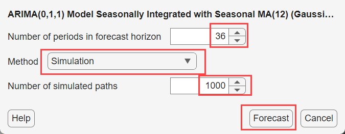
The right pane displays a figure window named FOR(SARIMA_PSSG_Log)_2 containing the series of log airline passenger counts, 3-year monthly Monte Carlo forecasts, and the 95% percentile intervals.
In the Forecasts pane, a variable named FOR_SARIMA_PSSG_Log_2 is a structure array containing the Monte Carlo forecasts, and the pointwise upper and lower percentile confidence bounds.
Export Session Results
Econometric Modeler offers several options for you to share your session results. The option you choose depends on your analysis goals.
The options for sharing your results are in the Export section of the Modeler tab. This table describes the available options.
| Option | Description |
|---|---|
Export Variables | Export time series and model variables to the MATLAB Workspace. Choose this option to perform further analysis at the MATLAB command line. For example, you can generate forecasts from an estimated model or check the predictive performance of several models. |
Generate Function | Generate a MATLAB function to use outside the app. The function accepts the data loaded into the app as input, and outputs a model estimated in the app session. Choose this option to:
|
| Generate Live Function | Generate a MATLAB live function to use outside the app. The function accepts the data loaded into the app as input, and outputs a model estimated in the app session. Choose this option to:
|
Generate Report | Generate a report that summarizes the session. Choose this option when you achieve your analysis goals in Econometric Modeler, and you want to share a summary of the results. |
Exporting Variables
To export variables, for example, time series, estimated model, or forecast variables, from the variable panes to the MATLAB Workspace:
On the Modeler tab, in the Export section, click
 or Export
> Export Variables.
or Export
> Export Variables.In the Export Data dialog box, choose variables to export by selecting the corresponding check boxes in the Select column. The app selects the check box of all variables that are selected in the variable panes. Clear any check boxes for variables to you do not want to export. For example, this figure shows how to select the
PSSG_Logtime series, theSARIMA_PSSG_LogSARIMA model, the MMSE forecast variableFOR_SARIMA_PSSG_Log, and the Monte Carlo forecastsFOR_SARIMA_PSSG_Log_2.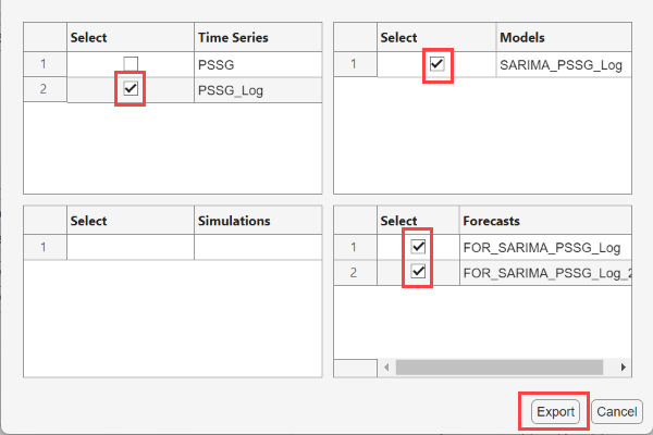
Click Export.
The selected variables appear in the MATLAB Workspace. Time series variables are double-precision column
vectors. Estimated models are objects of type depending on the model (for
example, an exported ARIMA model is an arima object).
Forecast variables are structure arrays with fields Forecast
containing a double-precision column vector of forecasts,
UpperConfidenceBound containing a double-precision column
vector of upper confidence bounds, and LowerConfidenceBound a
double-precision column vector of lower confidence bounds.
Alternatively, you can export variables by selecting at least one variable, right-clicking a selected variable, and selecting Export.
Generating a Function
The app can generate a plain text function or a live function. The main difference between the two functions is the editor used to modify the generated function: you edit plain text functions in the MATLAB editor and live functions in the Live Editor. For more details on the differences between the two function types, see What Is a Live Script or Function?.
Regardless of the function type you choose, the generated function accepts the data loaded into the app as input, and outputs the selected model, forecast, or simulation variable based on the input data, for example. To export a MATLAB function or live function that creates the selected model, forecast, or simulation variable in an app session:
The Models, Simulations, or Forecasts pane, select a variable.
On the Modeler tab, in the Export section, click the drop-down arrow. In the Export menu, choose Generate Function or Generate Live Function.
The MATLAB Editor or Live Editor displays an untitled, unsaved function containing the code that estimates the model.
By default, the function name is
typeTimeSeriestypeThe function accepts the originally imported data set as input.
Before the function computes the selected variable, it extracts the variables from the input data set used in estimation, and applies the same transformations to the variables that you applied in Econometric Modeler.
The function computes and returns the selected variable.
Consider generating a live function that returns the MMSE forecasts from
SARIMA_PSSG_Log, the
SARIMA(0,1,1)×(0,1,1)12 model fit to the log of the
airline passenger data (see Forecast Model with Best In-Sample Fit).
In the Forecasts pane, select the
FOR_SARIMA_PSSG_Logvariable.On the Modeler tab, in the Export section, click Export > Generate Live Function.
This figure shows the generated live function.

Generating a Report
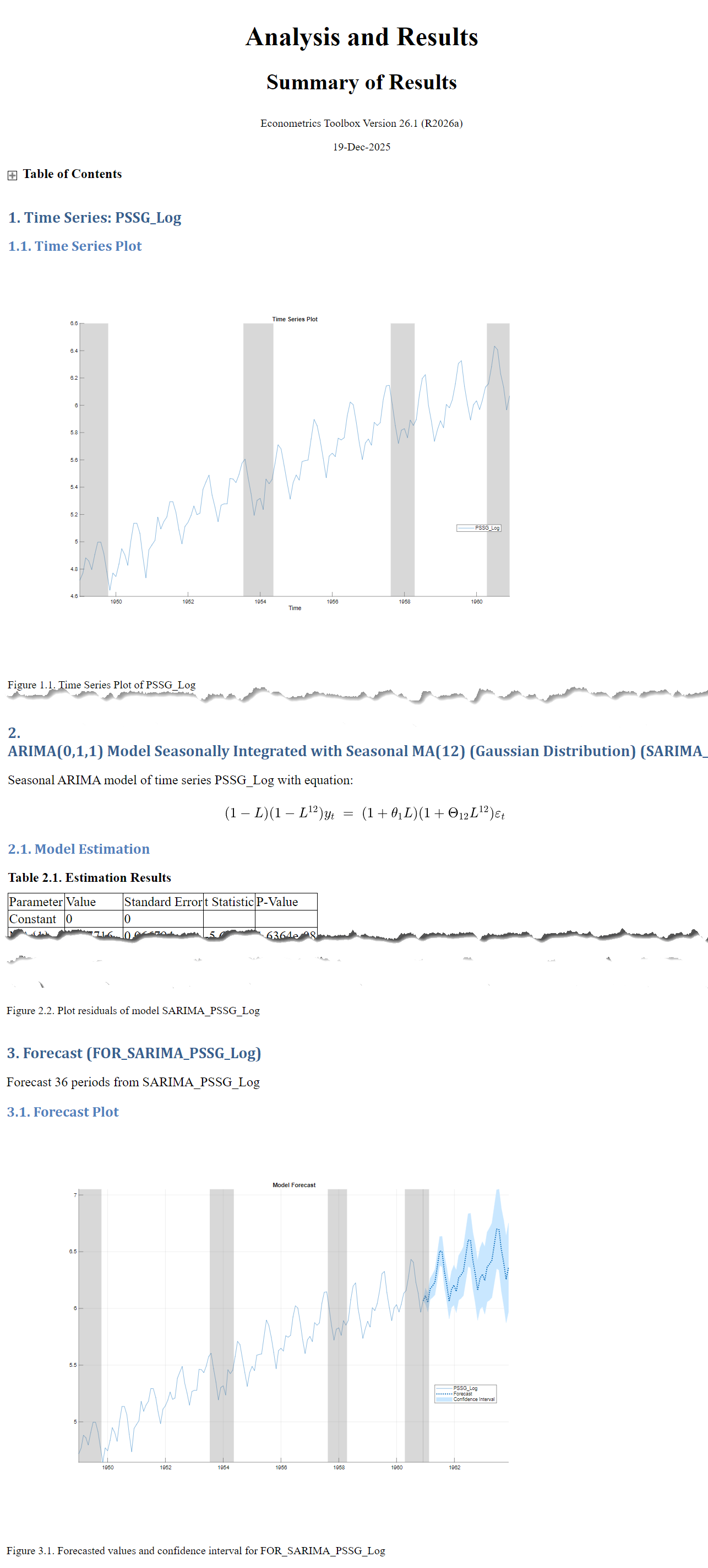
Econometric Modeler can produce a report describing your activities on selected time series and model variables. The app organizes the report into chapters corresponding to selected time series and model variables. Chapters describe session activities that you perform on the corresponding variable.
Chapters on time series variables describe transformations, plots, and tests that you perform on the selected variable in the session. Estimated model chapters contain an estimation summary, that is, elements of the Fit document (see Estimating a Univariate Model), residual diagnostics plots and tests, simulations from the model, and model forecasts.
You can export the report as one of the following document types:
Hypertext Markup Language (HTML)
Microsoft® Word XML Format Document (DOCX)
Portable Document Format (PDF)
To export a report:
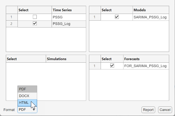
On the Modeler tab, in the Export section, click Export > Generate Report.
In the Generate Report dialog box, variables are categorized by type. Choose variables to include the report by selecting their check boxes in the Select column.
Select a document format by clicking Report Format and selecting the format.
Click Report.
In the Select File to Write window:
Browse to the folder in which you want to save the report.
In the File name box, type a name for the report.
Click Save.
Consider generating an HTML report for the analysis of the airline passenger data (see Conduct Goodness-of-Fit Checks). This figure shows how to select all variables and the HTML format.
This figure shows a sample of the generated report.
References
[1] Box, George E. P., Gwilym M. Jenkins, and Gregory C. Reinsel. Time Series Analysis: Forecasting and Control. 3rd ed. Englewood Cliffs, NJ: Prentice Hall, 1994.
See Also
Apps
Topics
- Prepare Time Series Data for Econometric Modeler App
- Import Time Series Data into Econometric Modeler App
- Plot Time Series Data Using Econometric Modeler App
- Detect Serial Correlation Using Econometric Modeler App
- Detect ARCH Effects Using Econometric Modeler App
- Assess Stationarity of Time Series Using Econometric Modeler
- Assess Collinearity Among Multiple Series Using Econometric Modeler App
- Conduct Cointegration Test Using Econometric Modeler
- Transform Time Series Using Econometric Modeler App
- Implement Box-Jenkins Model Selection and Estimation Using Econometric Modeler App
- Estimate Multiplicative ARIMA Model Using Econometric Modeler App
- Specify t Innovation Distribution Using Econometric Modeler App
- Perform ARIMA Model Residual Diagnostics Using Econometric Modeler App
- Estimate ARIMAX Model Using Econometric Modeler App
- Create Predictive Vector Autoregression Model Using Econometric Modeler
- Estimate Vector Error-Correction Model Using Econometric Modeler
- Compare Predictive Performance After Creating Models Using Econometric Modeler
- Estimate Regression Model with ARMA Errors Using Econometric Modeler App
- Select ARCH Lags for GARCH Model Using Econometric Modeler App
- Compare Conditional Variance Model Fit Statistics Using Econometric Modeler App
- Share Results of Econometric Modeler App Session
- Creating ARIMA Models Using Econometric Modeler App