Assess Stationarity of Time Series Using Econometric Modeler

These examples show how to conduct statistical hypothesis tests for assessing whether a time series is a unit root process by using the Econometric Modeler app. The test you use depends on your assumptions about the nature of the nonstationarity of an underlying model.

Test Assuming Unit Root Null Model

This example uses the Augmented Dickey-Fuller and Phillips-Perron tests to assess whether a time series is a unit root process. The null hypothesis for both tests is that the time series is a unit root process. The data set, stored in Data_USEconModel.mat, contains the US gross domestic product (GDP) measured quarterly, among other series.

At the command line, load the Data_USEconModel.mat data set.

load Data_USEconModel

At the command line, open the Econometric Modeler app.

econometricModeler

Alternatively, open the app from the apps gallery (see Econometric Modeler).

Import DataTimeTable into the app:

1. On the Econometric Modeler tab, in the Import section, click the Import button .

2. In the Import Data dialog box, in the Import? column, select the check box for the DataTimeTable variable.

3. Click Import.

The variables, among GDP, appear in the Time Series pane, and a time series plot of all the series appears in the Time Series Plot(COE) figure window.

In the Time Series pane, double-click GDP. A time series plot of GDP appears in the Time Series Plot(GDP) figure window.

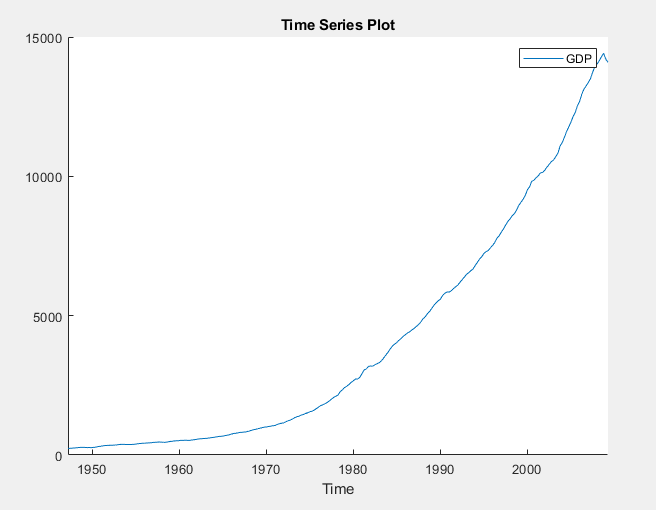
The series appears to grow without bound.

Apply the log transformation to GDP. On the Econometric Modeler tab, in the Transforms section, click Log.

In the Time Series pane, a variable representing the logged GDP (GDPLog) appears. A time series plot of the logged GDP appears in the Time Series Plot(GDPLog) figure window.

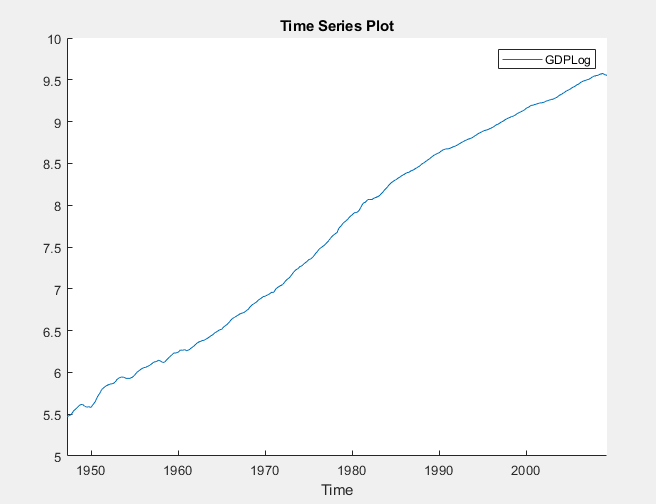
The logged GDP series appears to have a time trend or drift term.

Using the Augmented Dickey-Fuller test, test the null hypothesis that the logged GDP series has a unit root against a trend stationary AR(1) model alternative. Conduct a separate test for an AR(1) model with drift alternative. For the null hypothesis of both tests, include the restriction that the trend and drift terms, respectively, are zero by conducting F tests.

1. With GDPLog selected in the Time Series pane, on the Econometric Modeler tab, in the Tests section, click New Test > Augmented Dickey-Fuller Test.

2. On the ADF tab, in the Parameters section:

   1. Set Number of Lags to 1.

   2. Select Model > Trend Stationary.

   3. Select Test Statistic > F statistic.

3. In the Tests section, click Run Test.

4. Repeat steps 2 and 3, but select Model > Autoregressive with Drift instead.

The test results appear in the Results table of the ADF(GDPLog) document.

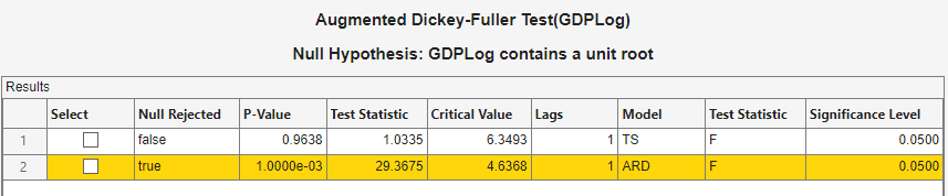
For the test supposing a trend stationary AR(1) model alternative, the null hypothesis is not rejected. For the test assuming an AR(1) model with drift, the null hypothesis is rejected.

Apply the Phillips-Perron test using the same assumptions as in the Augmented Dickey-Fuller tests, except the trend and drift terms in the null model cannot be zero.

1. With GDPLog selected in the Time Series pane, click the Econometric Modeler tab. Then, in the Tests section, click New Test > Phillips-Perron Test.

2. On the PP tab, in the Parameters section:

   1. Set Number of Lags to 1.

   2. Select Model > Trend Stationary.

3. In the Tests section, click Run Test.

4. Repeat steps 2 and 3, but select Model > Autoregressive with Drift instead.

The test results appear in the Results table of the PP(GDPLog) document.

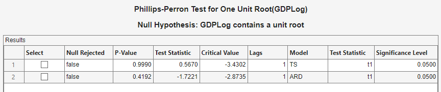
The null is not rejected for both tests. These results suggest that the logged GDP possibly has a unit root.

The difference in the null models can account for the differences between the Augmented Dickey-Fuller and Phillips-Perron test results.

Test Assuming Stationary Null Model

This example uses the Kwiatkowski, Phillips, Schmidt, and Shin (KPSS) test to assess whether a time series is a unit root process. The null hypothesis is that the time series is stationary. The data set, stored in Data_NelsonPlosser.mat, contains annual nominal wages, among other US macroeconomic series.

At the command line, load the Data_NelsonPlosser.mat data set.

load Data_NelsonPlosser

At the command line, open the Econometric Modeler app.

econometricModeler

Alternatively, open the app from the apps gallery (see Econometric Modeler).

Import DataTimeTable into the app:

1. On the Econometric Modeler tab, in the Import section, click the Import button .

2. In the Import Data dialog box, in the Import? column, select the check box for the DataTimeTable variable.

3. Click Import.

The variables, including the nominal wages WN, appear in the Time Series pane, and a time series plot of all the series appears in the Time Series Plot(BY)figure window.

In the Time Series pane, double-click WN. A time series plot of WN appears in the Time Series Plot(WN) figure window.

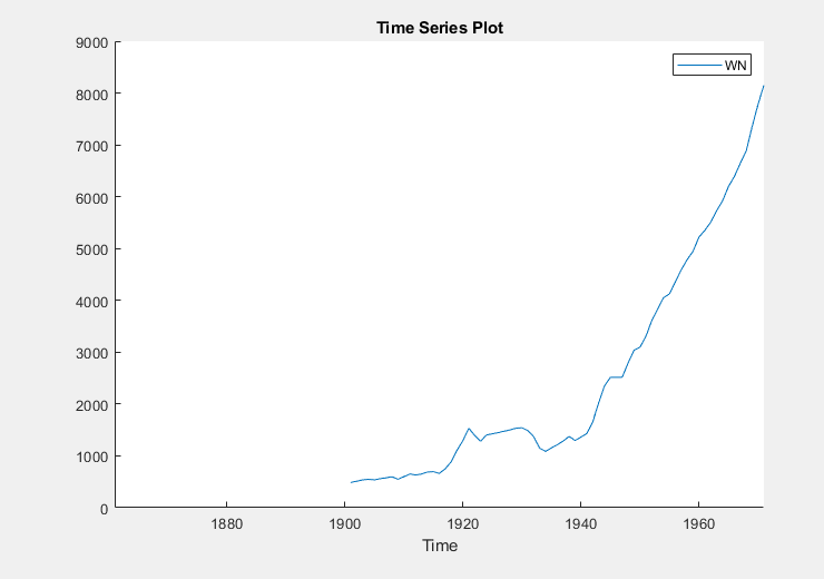
The series appears to grow without bound, and wage measurements are missing before 1900. To zoom into values occurring after 1900, pause on the plot, click , and enclose the time series in the box produced by dragging the cross hair.

Apply the log transformation to WN. On the Econometric Modeler tab, in the Transforms section, click Log.

In the Time Series pane, a variable representing the logged wages (WNLog) appears. The logged series appears in the Time Series Plot(WNLog) figure window.

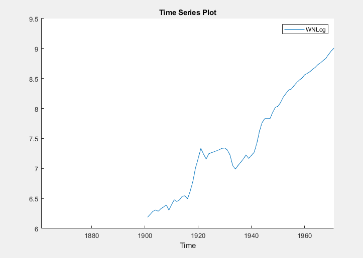
The logged wages appear to have a linear trend.

Using the KPSS test, test the null hypothesis that the logged wages are trend stationary against the unit root alternative. As suggested in [1], conduct three separate tests by specifying 7, 9, and 11 lags in the autoregressive model.

1. With WNLog selected in the Time Series pane, on the Econometric Modeler tab, in the Tests section, click New Test > KPSS Test.

2. On the KPSS tab, in the Parameters section, set Number of Lags to 7.

3. In the Tests section, click Run Test.

4. Repeat steps 2 and 3, but set Number of Lags to 9 instead.

5. Repeat steps 2 and 3, but set Number of Lags to 11 instead.

The test results appear in the Results table of the KPSS(WNLog) document.

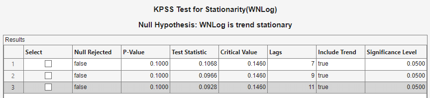
All tests fail to reject the null hypothesis that the logged wages are trend stationary.

Test Assuming Random Walk Null Model

This example uses the variance ratio test to assess the null hypothesis that a time series is a random walk. The data set, stored in CAPMuniverse.mat and available with the Financial Toolbox™ documentation, contains market data for daily returns of stocks and cash (money market) from the period January 1, 2000 to November 7, 2005.

At the command line, load the CAPMuniverse.mat data set.

load CAPMuniverse

The series are in the timetable AssetsTimeTable. The first column of data (AAPL) is the daily return of a technology stock. The last column is the daily return for cash (the daily money market rate, CASH).

Accumulate the daily technology stock and cash returns.

AssetsTimeTable.AAPLcumsum = cumsum(AssetsTimeTable.AAPL);
AssetsTimeTable.CASHcumsum = cumsum(AssetsTimeTable.CASH);

At the command line, open the Econometric Modeler app.

econometricModeler

Alternatively, open the app from the apps gallery (see Econometric Modeler).

Import AssetsTimeTable into the app:

1. On the Econometric Modeler tab, in the Import section, click .

2. In the Import Data dialog box, in the Import? column, select the check box for the AssetsTimeTable variable.

3. Click Import.

The variables, including stock and cash prices (AAPLcumsum and CASHcumsum), appear in the Time Series pane, and a time series plot of all the series appears in the Time Series Plot(AAPL) figure window.

In the Time Series pane, double-click AAPLcumsum. A time series plot of AAPLcumsum appears in the Time Series Plot(AAPLcumsum) figure window.

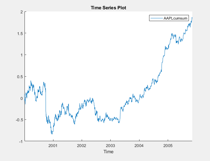
The accumulated returns of the stock appear to wander at first, with high variability, and then grow without bound after 2004.

Using the variance ratio test, test the null hypothesis that the series of accumulated stock returns is a random walk. First, test without assuming IID innovations for the alternative model, then test assuming IID innovations.

1. With AAPLcumsum selected in the Time Series pane, on the Econometric Modeler tab, in the Tests section, click New Test > Variance Ratio Test.

2. On the VRatio tab, in the Tests section, click Run Test.

3. On the VRatio tab, in the Parameters section, select the IID Innovations check box.

4. In the Tests section, click Run Test.

The test results appear in the Results table of the VRatio(AAPLcumsum) document.

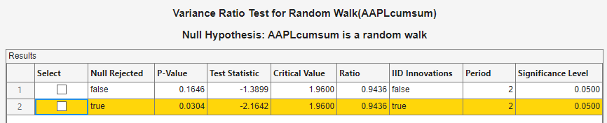
Without assuming IID innovations for the alternative model, the test fails to reject the random walk null model. However, assuming IID innovations, the test rejects the null hypothesis. This result might be due to heteroscedasticity in the series, that is, the series might be a heteroscedastic random walk.

In the Time Series pane, double-click CASHcumsum. A time series plot of CASHcumsum appears in the Time Series Plot(CASHcumsum) figure window.

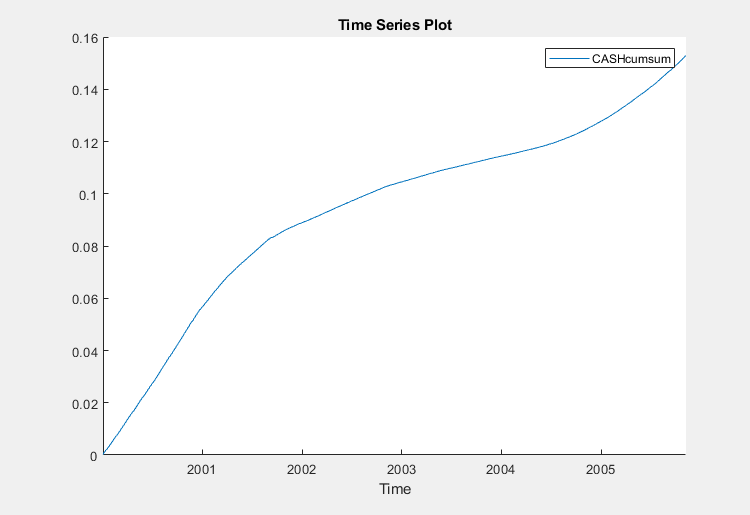
The series of accumulated cash returns exhibits low variability and appears to have long-term trends.

Test the null hypothesis that the series of accumulated cash returns is a random walk:

1. With CASHcumsum selected in the Time Series pane, on the Econometric Modeler tab, in the Tests section, click New Test > Variance Ratio Test.

2. On the VRatio tab, in the Parameters section, clear the IID Innovations box.

3. In the Tests section, click Run Test.

The test results appear in the Results tab of the VRatio(CASHcumsum) document.

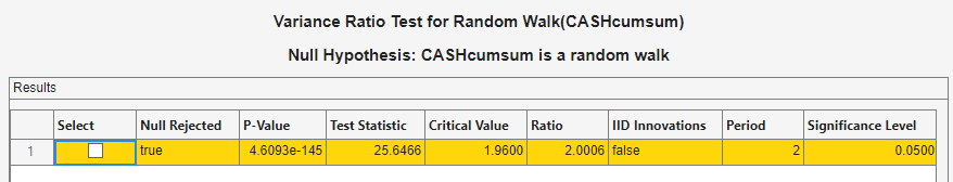
The test rejects the null hypothesis that the series of accumulated cash returns is a random walk.

References

[1] Kwiatkowski, D., P. C. B. Phillips, P. Schmidt, and Y. Shin. “Testing the Null Hypothesis of Stationarity against the Alternative of a Unit Root.” Journal of Econometrics. Vol. 54, 1992, pp. 159–178.