verifyEnsembleRobustness
R2026bVerify robustness of Statistics and Machine Learning Toolbox tree-based ensemble classifiers
Since R2026b
Syntax
Description
Add-On Required: This feature requires the AI Verification Library for Deep Learning Toolbox add-on.
results = verifyEnsembleRobustness(Mdl,TblLower,TblUpper,responseVarName)TblLower table and the upper bounds in the
TblUpper table.
For each region, the function verifies whether the expected class label in the
responseVarName variable matches the predicted class label returned
by the classification ensemble of trees Mdl. That is, the function
verifies whether Mdl is robust with respect to class label
i when the input is between TblLower(i,:) and
TblUpper(i,:). For more information, see Tree Ensemble Robustness.
The verifyEnsembleRobustness function requires Statistics and Machine Learning Toolbox™.
Examples
Verify the robustness of a classification ensemble of trees.
Load the humanactivity data set, which contains 24,075 observations of five different physical human activities: sitting, standing, walking, running, and dancing. Each observation has 60 features extracted from acceleration data measured by smartphone accelerometer sensors. Create a categorical variable (Activity) corresponding to the class labels for the observations, and convert the predictor data to a table (Tbl).
load humanactivity.mat
Activity = categorical(actid,1:5,actnames);
Tbl = array2table(feat,VariableNames=featlabels);
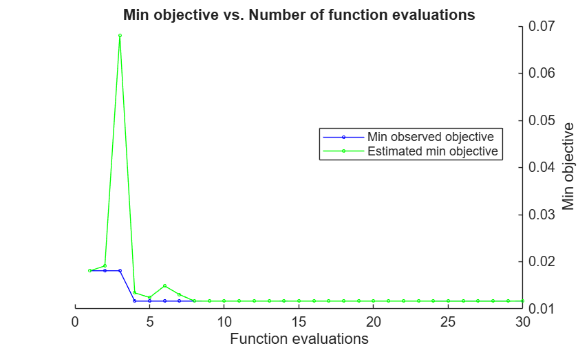
Train a classification ensemble of trees using the data. Tune the hyperparameters of the ensemble using Bayesian optimization with 3-fold cross-validation. The optimization process can take several minutes to run.
rng(0,"twister") % For reproducibility
hpoOptions = hyperparameterOptimizationOptions(KFold=3,Verbose=0);
Mdl = fitcensemble(Tbl,Activity,OptimizeHyperparameters="auto", ...
    HyperparameterOptimizationOptions=hpoOptions)
Mdl =
  ClassificationBaggedEnsemble
                       PredictorNames: {1×60 cell}
                         ResponseName: 'Y'
                CategoricalPredictors: []
                           ClassNames: [Sitting    Standing    Walking    Running    Dancing]
                       ScoreTransform: 'none'
                      NumObservations: 24075
    HyperparameterOptimizationResults: [1×1 classreg.learning.paramoptim.SupervisedLearningBayesianOptimization]
                           NumTrained: 229
                               Method: 'Bag'
                         LearnerNames: {'Tree'}
                 ReasonForTermination: 'Terminated normally after completing the requested number of training cycles.'
                              FitInfo: []
                   FitInfoDescription: 'None'
                            FResample: 1
                              Replace: 1
                     UseObsForLearner: [24075×229 logical]


  Properties, Methods
Create a region of predictor values on which to verify the predictive behavior of Mdl.
For each predictor, compute the mean and standard deviation of the observations corresponding to the activity of sitting. The lower bound of the region is the mean minus the standard deviation, and the upper bound of the region is the mean plus the standard deviation. Plot the lower and upper bounds.
sittingObservations = Tbl(Activity=="Sitting",:);

observationsMean = mean(sittingObservations);
observationsStd = std(sittingObservations);

tblLower = observationsMean - observationsStd;
tblUpper = observationsMean + observationsStd;

plot(tblLower{:,:})
hold on
plot(tblUpper{:,:})
hold off
legend("Lower bound","Upper bound")
xlabel("Predictor Index")
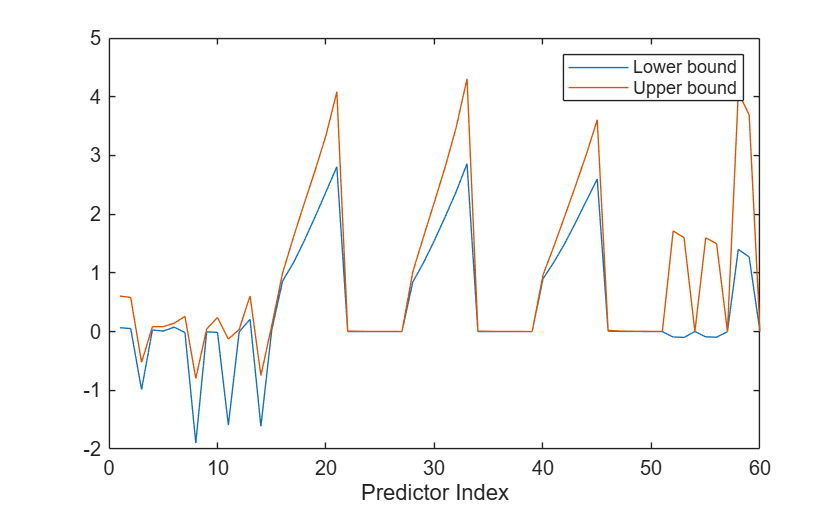
Verify that the ensemble predicts the class label Sitting for all observations in the region between tblLower and tblUpper.
result = verifyEnsembleRobustness(Mdl,tblLower,tblUpper,"Sitting")result = categorical
verified
Increase the perturbation region on which to verify the robustness of a classification ensemble of trees.
Load the carbig data set, which contains car measurements. First, convert Origin to a categorical variable with two categories, USA and NotUSA. Then, create a table from a subset of the variables. Include the categorical Origin variable.
load carbig

Origin = categorical(cellstr(Origin));
Origin = mergecats(Origin,["France","Japan","Germany", ...
    "Sweden","Italy","England"],"NotUSA");

cars = table(Acceleration,Displacement,Horsepower, ...
    Origin,MPG,Weight,Cylinders);
Train a classification ensemble using the data in cars. Specify Cylinders as the response variable. Ensure that Mdl is an ensemble of trees.
Mdl = fitcensemble(cars,"Cylinders",Learners="tree")
Mdl =
  ClassificationEnsemble
           PredictorNames: {'Acceleration'  'Displacement'  'Horsepower'  'Origin'  'MPG'  'Weight'}
             ResponseName: 'Cylinders'
    CategoricalPredictors: 4
               ClassNames: [3 4 5 6 8]
           ScoreTransform: 'none'
          NumObservations: 406
               NumTrained: 100
                   Method: 'AdaBoostM2'
             LearnerNames: {'Tree'}
     ReasonForTermination: 'Terminated normally after completing the requested number of training cycles.'
                  FitInfo: [100×1 double]
       FitInfoDescription: {2×1 cell}


  Properties, Methods
Select an observation from the data. Check the class label that Mdl predicts for the observation.
idx = 1;
observation = cars(idx,:)
observation = 1×7 table
    Acceleration    Displacement    Horsepower    Origin    MPG    Weight    Cylinders
    ____________    ____________    __________    ______    ___    ______    _________

         12             307            130         USA      18      3504         8
predictedLabel = predict(Mdl,observation)
predictedLabel =
8
Perturb the observation by increasing amounts. Note that you can perturb only numeric predictor values; categorical values must be the same for the lower and upper bounds.
To perturb the numeric predictor values, use the custom perturbPredictors function, which accepts numeric predictor data (numericPredictors) and a percentage (percent). For each predictor, the function computes the specified percentage of the interquartile range and returns the value (perturbation).
function perturbation = perturbPredictors(numericPredictors,percent)
perturbation = percent*iqr(numericPredictors);
end
Increase the perturbation by increasing the percentage value from 5% to 25% in increments of 5%. Create a lower bound for the observation by subtracting the perturbation value, and create an upper bound by adding the perturbation value. Combine all the lower bounds in TblLower, and combine all the upper bounds in TblUpper.
numericPredictorNames = Mdl.PredictorNames;
numericPredictorNames(Mdl.CategoricalPredictors) = [];

percentRange = 0.05:0.05:0.25;
TblLower = repmat(observation,numel(percentRange),1);
TblUpper = TblLower;

for k = 1:numel(percentRange)
    percentk = percentRange(k);
    perturbk = @(numericPredictors)perturbPredictors(numericPredictors,percentk);
    perturbationk = varfun(perturbk,cars, ...
        InputVariables=numericPredictorNames);
    perturbationk.Properties.VariableNames = numericPredictorNames;

    TblLower(k,numericPredictorNames) = ...
        TblLower(k,numericPredictorNames) - perturbationk;

    TblUpper(k,numericPredictorNames) = ...
        TblUpper(k,numericPredictorNames) + perturbationk;
end
Verify the robustness of the model on the increasing perturbation regions.
results = verifyEnsembleRobustness(Mdl,TblLower,TblUpper,"Cylinders")results = 5×1 categorical
verified
verified
verified
verified
violated
In the first four perturbation regions, Mdl predicts the same class label (8) for all observations with values between the lower and upper bounds. In the last perturbation region, Mdl predicts a different class label (3, 4, 5, or 6) for at least one combination of predictor values between the lower bound TblLower(5,:) and the upper bound TblUpper(5,:).
Input Arguments
Output Arguments
Tips
Expect the verification process to take longer for more complex ensembles. For more information on how the performance of
verifyEnsembleRobustnessdepends on the structure of the ensemble, see Performance.
Algorithms
References
[1] Matsunaga, Saori, and Genta Yoshimura. “Efficient and High-Quality Formal Verification for Decision Tree Ensembles.” 2024 IEEE International Conference on Data Mining Workshops (ICDMW), December 9, 2024, 51–58. https://doi.org/10.1109/ICDMW65004.2024.00013.
[2] Ranzato, Francesco, and Marco Zanella. “Abstract Interpretation of Decision Tree Ensemble Classifiers.” Proceedings of the AAAI Conference on Artificial Intelligence 34, no. 04 (2020): 5478–86. https://doi.org/10.1609/aaai.v34i04.5998.
Version History
Introduced in R2026b
See Also
fitcensemble (Statistics and Machine Learning Toolbox) | verifyTreeRobustness | verifyNetworkRobustness

