comm.AWGNChannel
Add white Gaussian noise to input signal
Description
comm.AWGNChannel adds white Gaussian noise to the input signal.
When applicable, if inputs to the object have a variable number of channels, the EbNo, EsNo, SNR, BitsPerSymbol, SignalPower, SamplesPerSymbol, and Variance properties must be scalars.
To add white Gaussian noise to an input signal:
Create the
comm.AWGNChannelobject and set its properties.Call the object with arguments, as if it were a function.
To learn more about how System objects work, see What Are System Objects?
Creation
Description
awgnchan = comm.AWGNChannelawgnchan. This object then adds white Gaussian noise to a
real or complex input signal.
awgnchan = comm.AWGNChannel(Name,Value)awgnchan, with the specified property
Name set to the specified Value. You can specify
additional name-value pair arguments in any order as
(Name1,Value1,...,NameN,ValueN).
Properties
Usage
Description
outsignal = awgnchan(insignal,var)'Variance' and VarianceSource to 'Input
port'.
For example:
awgnchan = comm.AWGNChannel('NoiseMethod','Variance', ...
     'VarianceSource','Input port');
var = 12;
...
outsignal = awgnchan(insignal,var);Input Arguments
Output Arguments
Object Functions
To use an object function, specify the
System object as the first input argument. For
example, to release system resources of a System object named obj, use
this syntax:
release(obj)
Examples
Create an AWGN channel System object with the default configuration. Pass signal data through this channel.
Create an AWGN channel object and signal data.
awgnchan = comm.AWGNChannel;
insignal = randi([0 1],100,1);
Send the input signal through the channel.
outsignal = awgnchan(insignal);
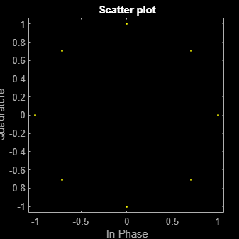
Modulate an 8-PSK signal, add white Gaussian noise, and plot the signal to visualize the effects of the noise.
Modulate the signal.
modData = pskmod(randi([0 7],2000,1),8);
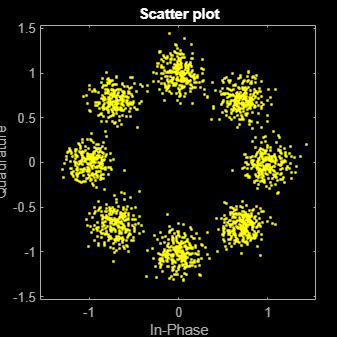
Add white Gaussian noise to the modulated signal by passing the signal through an additive white Gaussian noise (AWGN) channel.
channel = comm.AWGNChannel('EbNo',20,'BitsPerSymbol',3);
Transmit the signal through the AWGN channel.
channelOutput = channel(modData);
Plot the noiseless and noisy data by using scatter plots to visualize the effects of the noise.
scatterplot(modData)
scatterplot(channelOutput)

Change the EbNo property to 10 dB to increase the noise.
channel.EbNo = 10;
Pass the modulated data through the AWGN channel.
channelOutput = channel(modData);
Plot the channel output. You can see the effects of increased noise.
scatterplot(channelOutput)
To accurately represent the noise level the bit energy to noise density ratio (Eb/No) for communication links must account for the bits per symbol and coding rate of the signal transmitted through the channel.
Define the codeword and message length for a Reed-Solomon code and the modulation order of the signal.
N = 15;         % R-S codeword length in symbols
K = 9;          % R-S message length in symbols
codeRate = K/N; % R-S code rate
M = 16;         % Modulation order
bps = log2(M);  % Bits per symbol
Specify the uncoded Eb/No in dB. Convert the uncoded Eb/No to the corresponding coded Eb/No using the code rate.
UncodedEbNo = 6;
CodedEbNo = UncodedEbNo + 10*log10(codeRate);
Construct an AWGN channel object setting the number of bits per symbol and the coded Eb/No.
channel1 = comm.AWGNChannel( ...
    NoiseMethod='Signal to noise ratio (Eb/No)', ...
    BitsPerSymbol=bps, ...
    EbNo=CodedEbNo)
channel1 =
  comm.AWGNChannel with properties:

         NoiseMethod: 'Signal to noise ratio (Eb/No)'
                EbNo: 3.7815
       BitsPerSymbol: 4
         SignalPower: 1
    SamplesPerSymbol: 1
        RandomStream: 'Global stream'
For an alternative approach, you can convert the uncoded Eb/No to the corresponding SNR, and then configure an AWGN channel object setting noise method to SNR.
snr = convertSNR(UncodedEbNo,"ebno","SNR", ...
    BitsPerSymbol=bps, ...
    CodingRate=codeRate);
channel2 = comm.AWGNChannel( ...
    NoiseMethod='Signal to noise ratio (SNR)', ...
    SNR=snr)
channel2 =
  comm.AWGNChannel with properties:

     NoiseMethod: 'Signal to noise ratio (SNR)'
             SNR: 9.8021
     SignalPower: 1
    RandomStream: 'Global stream'
Pass a single-channel and multichannel signal through an AWGN channel System object™.
Create an AWGN channel System object with the Eb/No ratio set for a single channel input. In this case, the EbNo property is a scalar.
channel = comm.AWGNChannel('EbNo',15);Generate random data and apply QPSK modulation.
data = randi([0 3],1000,1);
modData = pskmod(data,4,pi/4);
Pass the modulated data through the AWGN channel.
rxSig = channel(modData);
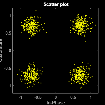
Plot the noisy constellation.
scatterplot(rxSig)
Generate two-channel input data and apply QPSK modulation.
data = randi([0 3],2000,2);
modData = pskmod(data,4,pi/4);
Pass the modulated data through the AWGN channel.
rxSig = channel(modData);
Plot the noisy constellations. Each channel is represented as a single column in rxSig. The plots are nearly identical, because the same Eb/No value is applied to both channels.
scatterplot(rxSig(:,1))
title('First Channel')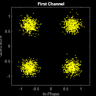
scatterplot(rxSig(:,2))
title('Second Channel')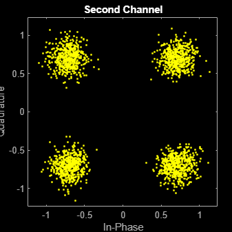
Modify the AWGN channel object to apply a different Eb/No value to each channel. To apply different values, set the EbNo property to a 1-by-2 vector. When changing the dimension of the EbNo property, you must release the AWGN channel object.
release(channel)
channel.EbNo = [10 20];
Pass the data through the AWGN channel.
rxSig = channel(modData);
Plot the noisy constellations. The first channel has significantly more noise due to its lower Eb/No value.
scatterplot(rxSig(:,1))
title('First Channel')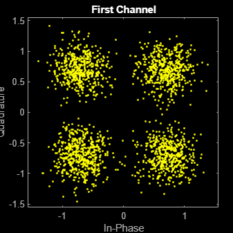
scatterplot(rxSig(:,2))
title('Second Channel')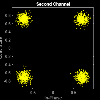
Apply the noise variance input as a scalar or a row vector, with a length equal to the number of channels of the current signal input.
Create an AWGN channel System object™ with the NoiseMethod property set to 'Variance' and the VarianceSource property set to 'Input port'.
channel = comm.AWGNChannel('NoiseMethod','Variance', ...
'VarianceSource','Input port');
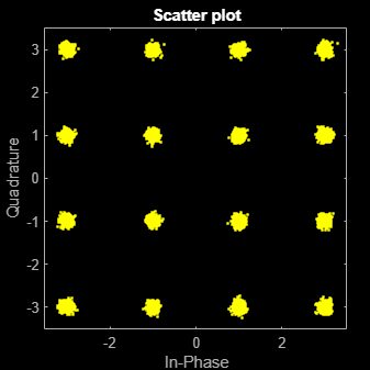
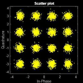
Generate random data for two channels and apply 16-QAM modulation.
data = randi([0 15],10000,2);
txSig = qammod(data,16);
Pass the modulated data through the AWGN channel. The AWGN channel object processes data from two channels. The variance input is a 1-by-2 vector.
rxSig = channel(txSig,[0.01 0.1]);
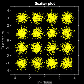
Plot the constellation diagrams for the two channels. The second signal is noisier because its variance is ten times larger.
scatterplot(rxSig(:,1))
scatterplot(rxSig(:,2))
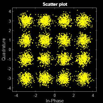
Repeat the process where the noise variance input is a scalar. The same variance is applied to both channels. The constellation diagrams are nearly identical.
rxSig = channel(txSig,0.2);
scatterplot(rxSig(:,1))
scatterplot(rxSig(:,2))
Specify a seed to produce the same outputs when using a random stream in which you specify the seed.
Create an AWGN channel System object™. Set the NoiseMethod property to 'Variance', the RandomStream property to 'mt19937ar with seed', and the Seed property to 99.
channel = comm.AWGNChannel( ...
    'NoiseMethod','Variance', ...
    'RandomStream','mt19937ar with seed', ...
    'Seed',99);
Pass data through the AWGN channel.
y1 = channel(zeros(8,1));
Pass another all-zeros vector through the channel.
y2 = channel(zeros(8,1));
Because the seed changes between function calls, the output is different.
isequal(y1,y2)
ans = logical
   0
Reset the AWGN channel object by calling the reset function. The random data stream is reset to the initial seed of 99.
reset(channel);
Pass the all-zeros vector through the AWGN channel.
y3 = channel(zeros(8,1));
Confirm that the two signals are identical.
isequal(y1,y3)
ans = logical
   1
Algorithms
References
[1] Proakis, John G. Digital Communications. 4th Ed. McGraw-Hill, 2001.
Extended Capabilities
Version History
Introduced in R2012a