comm.RicianChannel
Filter input signal through multipath Rician fading channel
Description
The comm.RicianChannel
System object™ filters an input signal through a multipath Rician fading channel. For more
information on fading model processing, see the Methodology for Simulating
Multipath Fading Channels section.
To filter an input signal through a multipath Rician fading channel:
Create the
comm.RicianChannelobject and set its properties.Call the object with arguments, as if it were a function.
To learn more about how System objects work, see What Are System Objects?
Creation
Description
ricianchan = comm.RicianChannel
ricianchan = comm.RicianChannel(Name=Value)comm.RicianChannel(SampleRate=2) sets the input signal sample rate to
2.
Properties
Usage
Syntax
Description
Y = ricianchan(X)X through a multipath Rician fading channel
and returns the result in Y.
To enable this syntax, set the ChannelFiltering property
to true.
Y = ricianchan(X,inittime)
To enable this syntax, set the FadingTechnique property to
'Sum of sinusoids' and the InitialTimeSource
property to 'Input port'.
[
also returns the channel path gains of the underlying multipath Rician fading process in
Y,pathgains] = ricianchan(___)pathgains using any of the input argument combinations in the
previous syntaxes.
To enable this syntax, set the PathGainsOutputPort
property to true.
pathgains = ricianchan()
To enable this syntax, set the ChannelFiltering property
to false.
pathgains = ricianchan(inittime)
To enable this syntax, set the FadingTechnique property to
'Sum of sinusoids', the InitialTimeSource
property to 'Input port', and the ChannelFiltering property
to false.
Input Arguments
Output Arguments
Object Functions
To use an object function, specify the
System object as the first input argument. For
example, to release system resources of a System object named obj, use
this syntax:
release(obj)
Examples
Produce the same multipath Rician fading channel response by using two different methods for random number generation. The multipath Rician fading channel System object includes two methods for random number generation. You can use the current global stream or the mt19937ar algorithm with a specified seed. By interacting with the global stream, the System object can produce the same outputs from the two methods.
Apply 8-PSK modulation to randomly generated data.
M = 8; % Modulation order
insig = randi([0,M-1],1024,1);
channelInput = pskmod(insig,M);
Create a multipath Rician fading channel System object, specifying the random number generation method as the my19937ar algorithm and the random number seed as 73.
ricianchan = comm.RicianChannel( ...
    SampleRate=1e6, ...
    PathDelays=[0.0 0.5 1.2]*1e-6, ...
    AveragePathGains=[0.1 0.5 0.2], ...
    KFactor=2.8, ...
    DirectPathDopplerShift=5.0, ...
    DirectPathInitialPhase=0.5, ...
    MaximumDopplerShift=50, ...
    DopplerSpectrum=doppler('Bell', 8), ...
    RandomStream='mt19937ar with seed', ...
    Seed=73, ...
    PathGainsOutputPort=true);
Filter the modulated data by using the multipath Rician fading channel System object.
[RicianChanOut1,RicianPathGains1] = ricianchan(channelInput);
Set the System object to use the global stream for random number generation.
release(ricianchan);
ricianchan.RandomStream = 'Global stream';
Set the global stream to have the same seed that you specified when creating the multipath Rician fading channel System object.
rng(73)
Filter the modulated data by using the multipath Rician fading channel System object again.
[RicianChanOut2,RicianPathGains2] = ricianchan(channelInput);
Verify that the channel and path gain outputs are the same for each of the two methods.
isequal(RicianChanOut1,RicianChanOut2)
ans = logical
   1
isequal(RicianPathGains1,RicianPathGains2)
ans = logical
   1
Produce the multipath Rician fading channel response by using two different path gain sampling rates. The multipath Rician fading channel System object allows you to set the path gain sampling rate equal to the signal sampling rate or a lower rate computed based on the configuration of the object.
Apply 32-QAM modulation to randomly generated data.
M = 32;
spf = 2^12;
insig = randi([0,M-1],spf,1);
channelInput = qammod(insig,M);
numFrames = 2e4;
Create a multipath Rician fading channel System object with three paths. Before comparing the execution times, run once to load the object.
ricianchan = comm.RicianChannel( ...
    SampleRate=20e6, ...
    PathDelays=[0 1.5e-7 1.5e-7], ...
    AveragePathGains=[2 3 5], ...
    NormalizePathGains=true, ...
    KFactor=[3 2 4], ...
    DirectPathDopplerShift=[0 2 5], ...
    DirectPathInitialPhase=[0 pi/4 pi/7], ...
    MaximumDopplerShift=30, ...
    DopplerSpectrum= ...
        {doppler('Jakes'),doppler('Flat'),doppler('Bell')}, ...
    RandomStream='mt19937ar with seed', ...
    Seed=22, ...
    PathGainsOutputPort=true)
ricianchan =
  comm.RicianChannel with properties:

                SampleRate: 20000000
        PathGainSampleRate: 'signal'
                PathDelays: [0 1.5000e-07 1.5000e-07]
          AveragePathGains: [2 3 5]
        NormalizePathGains: true
                   KFactor: [3 2 4]
    DirectPathDopplerShift: [0 2 5]
    DirectPathInitialPhase: [0 0.7854 0.4488]
       MaximumDopplerShift: 30
           DopplerSpectrum: {[1×1 struct]  [1×1 struct]  [1×1 struct]}
          ChannelFiltering: true
       PathGainsOutputPort: true

  Show all properties
ricianchan(channelInput);
Use the info object function to show the configuration. Filter the modulated data by using the multipath Rician fading channel System object. Show the time required to filter a number of frames of data with the path gain sampling rate equal to the signal sampling rate.
info(ricianchan)
ans = struct with fields:
    ChannelFilterCoefficients: [3×4 double]
           ChannelFilterDelay: 0
          NumSamplesProcessed: 4096
           PathGainSampleRate: 20000000
tic
for ii = 1:numFrames
    [chanOut1,pathGains1] = ricianchan(channelInput);
end
toc
Elapsed time is 7.797282 seconds.
Release the object and change the PathGainSampleRate to 'auto'. Use the info object function to show the configuration. Repeat the Rician channel filtering of the modulated data and show the time required to filter the same number of frames of data with the lower path gain sampling rate computed by the object.
release(ricianchan);
ricianchan.PathGainSampleRate = 'auto'
ricianchan =
comm.RicianChannel with properties:
SampleRate: 20000000
PathGainSampleRate: 'auto'
PathDelays: [0 1.5000e-07 1.5000e-07]
AveragePathGains: [2 3 5]
NormalizePathGains: true
KFactor: [3 2 4]
DirectPathDopplerShift: [0 2 5]
DirectPathInitialPhase: [0 0.7854 0.4488]
MaximumDopplerShift: 30
DopplerSpectrum: {[1×1 struct] [1×1 struct] [1×1 struct]}
ChannelFiltering: true
PathGainsOutputPort: true
Show all properties
ricianchan(channelInput);
info(ricianchan)
ans = struct with fields:
    ChannelFilterCoefficients: [3×4 double]
           ChannelFilterDelay: 0
          NumSamplesProcessed: 4096
           PathGainSampleRate: 300.0030
tic
for ii = 1:numFrames
    [chanOut2,pathGains2] = ricianchan(channelInput);
end
toc
Elapsed time is 2.453173 seconds.
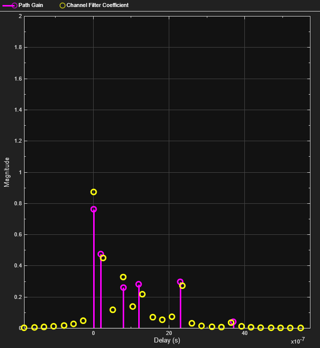
Display the impulse and frequency responses of a frequency-selective multipath Rician fading channel that is configured to disable channel filtering.
Define simulation variables. Specify path delays and gains by using the ITU pedestrian B channel configuration.
fs = 3.84e6;                                  % Sample rate in Hz
pathDelays = [0 200 800 1200 2300 3700]*1e-9; % in seconds
avgPathGains = [0 -0.9 -4.9 -8 -7.8 -23.9];   % dB
kfact = 10;                                   % Rician K-factor
fD = 50;                                      % Max Doppler shift in Hz
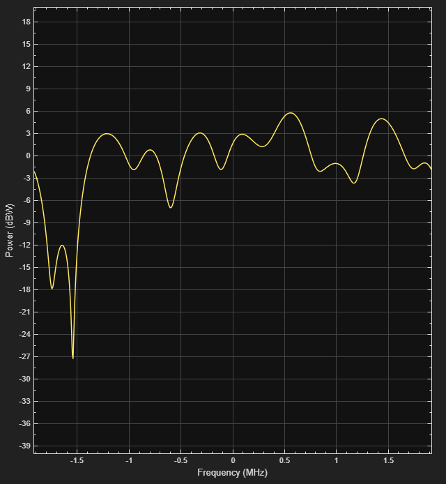
Create a multipath Rician fading channel System object to visualize the impulse response and frequency response plots.
ricianChan = comm.RicianChannel( ...
    SampleRate=fs, ...
    PathDelays=pathDelays, ...
    AveragePathGains=avgPathGains, ...
    KFactor=kfact, ...
    MaximumDopplerShift=fD, ...
    ChannelFiltering=false, ...
    Visualization='Impulse and frequency responses');
Visualize the channel response by running the multipath Rician fading channel System object with no input signal. The impulse response plot enables you to identify the individual paths and their corresponding filter coefficients. The frequency response plot shows the frequency-selective nature of the ITU pedestrian B channel.
ricianChan();
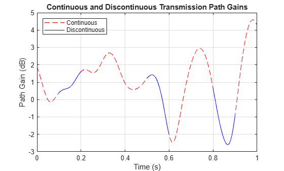
Show that the channel state is maintained for discontinuous transmissions by using multipath Rician fading channel System objects configured to use the sum-of-sinusoids fading technique. Observe discontinuous channel response segments overlaid on a continuous channel response.
Set the channel properties.
fs = 1000;               % Sample rate in Hz
pathDelays = [0 2.5e-3]; % In seconds
pathPower = [0 -6];      % In dB
fD = 5;                  % Maximum Doppler shift in Hz
ns = 1000;               % Number of samples
nsdel = 100;             % Number of samples for delayed paths
Define a continuous time span and three discontinuous time segments over which to plot and view the channel response. View a 1000-sample continuous channel response that starts at time 0 and three 100-sample channel responses that start at times 0.1, 0.4, and 0.7 seconds, respectively.
to0 = 0.0;
to1 = 0.1;
to2 = 0.5;
to3 = 0.8;
t0 = (to0:ns-1)/fs;      % Transmission 0
t1 = to1+(0:nsdel-1)/fs; % Transmission 1
t2 = to2+(0:nsdel-1)/fs; % Transmission 2
t3 = to3+(0:nsdel-1)/fs; % Transmission 3
Create a frequency-flat multipath Rician fading System object, specifying a 1000 Hz sampling rate, the sum-of-sinusoids fading technique, disabled channel filtering, and the number of samples to view. Specify a seed value so that results can be repeated. Use the default InitialTime property setting so that the fading channel is simulated from time 0.
ricianchan1 = comm.RicianChannel('SampleRate',fs, ...
    'MaximumDopplerShift',fD, ...
    'RandomStream','mt19937ar with seed', ...
    'Seed',17, ...
    'FadingTechnique','Sum of sinusoids', ...
    'ChannelFiltering',false, ...
    'NumSamples',ns);
Create a clone of the multipath Rician fading channel System object. Set the number of samples for the delayed paths. Set the source for the initial time so that you can specify the fading channel offset time as an input argument when using the System object.
ricianchan2 = clone(ricianchan1);
ricianchan2.InitialTimeSource = 'Input port';
ricianchan2.NumSamples = nsdel;
Save the path gain output for the continuous channel response by using the ricianchan1 object and for the discontinuous delayed channel responses by using the ricianchan2 object with the initial time offsets provided as input arguments.
pg0 = ricianchan1();
pg1 = ricianchan2(to1);
pg2 = ricianchan2(to2);
pg3 = ricianchan2(to3);
Compare the number of samples processed by the two channels by using the info object function. The ricianchan1 object processed 1000 samples, while the ricianhan2 object processed only 300 samples.
G = info(ricianchan1);
H = info(ricianchan2);
[G.NumSamplesProcessed H.NumSamplesProcessed]
ans = 1×2

        1000         300
Convert the path gains into decibels.
pathGain0 = 20*log10(abs(pg0));
pathGain1 = 20*log10(abs(pg1));
pathGain2 = 20*log10(abs(pg2));
pathGain3 = 20*log10(abs(pg3));
Plot the path gains for the continuous and discontinuous cases. The gains for the three segments match the gain for the continuous case. Because the channel characteristics are maintained even when data is not transmitted, the alignment of the two plots shows that the sum-of-sinusoids technique is suited to the simulation of packetized data.
plot(t0,pathGain0,'r--')
hold on
plot(t1,pathGain1,'b')
plot(t2,pathGain2,'b')
plot(t3,pathGain3,'b')
grid
xlabel('Time (s)')
ylabel('Path Gain (dB)')
legend('Continuous','Discontinuous','location','nw')
title('Continuous and Discontinuous Transmission Path Gains')
Reproduce the multipath Rician fading channel output by using the ChannelFilterCoefficients property returned by the info object function of the comm.RicianChannel System object.
Create a multipath Rician fading channel System object, defining two paths. Generate data to pass through the channel.
ricianchan = comm.RicianChannel( ...
    'SampleRate',1000, ...
    'PathDelays',[0 1e-3], ...
    'AveragePathGains',[0 -2], ...
    'PathGainsOutputPort',true)
ricianchan =
  comm.RicianChannel with properties:

                SampleRate: 1000
        PathGainSampleRate: 'signal'
                PathDelays: [0 1.0000e-03]
          AveragePathGains: [0 -2]
        NormalizePathGains: true
                   KFactor: 3
    DirectPathDopplerShift: 0
    DirectPathInitialPhase: 0
       MaximumDopplerShift: 1.0000e-03
           DopplerSpectrum: [1×1 struct]
          ChannelFiltering: true
       PathGainsOutputPort: true

  Show all properties
data = randi([0 1],600,1);
Pass data through the channel. Assign the ChannelFilterCoefficients property value to the variable coeff.
[chanout1,pg] = ricianchan(data);
chaninfo = info(ricianchan)
chaninfo = struct with fields:
    ChannelFilterCoefficients: [2×2 double]
           ChannelFilterDelay: 0
          NumSamplesProcessed: 600
           PathGainSampleRate: 1000
coeff = chaninfo.ChannelFilterCoefficients;
Calculate the fractional delayed input signal at the path delay locations stored in coeff.
Np = length(ricianchan.PathDelays);
fracdelaydata = zeros(size(data,1),Np);
for ii = 1:Np
    fracdelaydata(:,ii) = filter(coeff(ii,:),1,data);
end
Apply the path gains and sum the results for all paths.
chanout2 = sum(pg .* fracdelaydata,2);
Compare the output of the multipath Rician fading channel System object to the output reproduced using the path gains and the ChannelFilterCoefficients property of the multipath Rician fading channel System object.
isequal(chanout1,chanout2)
ans = logical
   1
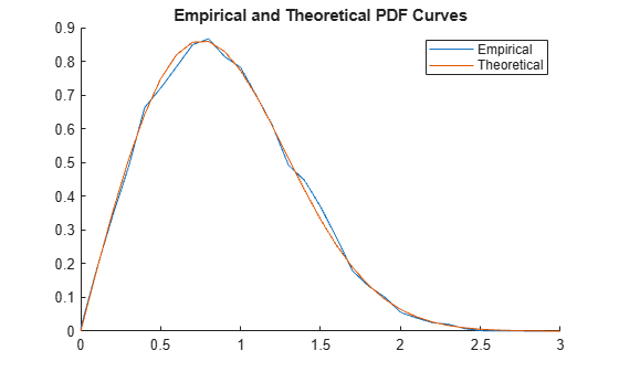
Compute and plot the empirical and theoretical probability density function (PDF) for a Rician channel with one path.
Initialize parameters and create a Rician channel System object that does not apply channel filtering.
Ns = 1.92e6;
Rs = 1.92e6;
dopplerShift = 2000;
KFactor = -3;                  % In dB
KFactorLin = 10.^(KFactor/10); % Linear units

chan = comm.RicianChannel( ...
    'SampleRate',Rs, ...
    'PathDelays',0, ...
    'KFactor',KFactorLin, ...
    'AveragePathGains',0, ...
    'MaximumDopplerShift',dopplerShift, ...
    'ChannelFiltering',false, ...
    'NumSamples',Ns, ...
    'FadingTechnique','Sum of sinusoids');
Compute and plot the empirical and theoretical PDF for the Rician channel, by using the fitdist (Statistics and Machine Learning Toolbox) and pdf (Statistics and Machine Learning Toolbox) functions.
figure;
hold on;

% Empirical PDF plot
gain = chan();
pd = fitdist(abs(gain),'Kernel','BandWidth',.01);
r = 0:.1:3;
y = pdf(pd,r);
plot(r,y)

% Theoretical PDF plot
s = sqrt(KFactorLin)/sqrt(KFactorLin+1);
sigma = sqrt(1/2)/sqrt(KFactorLin+1);
exp_pdf_amplitude = pdf('Rician',r,s,sigma);
plot(r,exp_pdf_amplitude')
legend('Empirical','Theoretical')
title('Empirical and Theoretical PDF Curves')
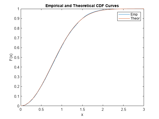
Compute and plot the empirical and theoretical cumulative distribution function (CDF) for a Rician channel with one path.
Initialize parameters and create a Rician channel System object that does not perform channel filtering.
Ns = 1.92e6;
Rs = 1.92e6;
dopplerShift = 2000;
KFactor = -3;                  % In dB
KFactorLin = 10.^(KFactor/10); % Linear units

chan = comm.RicianChannel( ...
    'SampleRate',Rs, ...
    'PathDelays',0, ...
    'KFactor',KFactorLin, ...
    'AveragePathGains',0, ...
    'MaximumDopplerShift',dopplerShift, ...
    'ChannelFiltering',false, ...
    'NumSamples',Ns, ...
    'FadingTechnique','Sum of sinusoids');
Compute and plot the empirical and theoretical CDF for the Rician channel by using the ecdf (Statistics and Machine Learning Toolbox) and cdf (Statistics and Machine Learning Toolbox) functions. Compute the empirical CDF by using the path gains.
% Empirical CDF plot
g = chan();
ecdf(abs(g));
hold on;

% Theoretical CDF plot
r = 0:.1:3;
s = sqrt(KFactorLin)/sqrt(KFactorLin+1);
sigma = sqrt(1/2)/sqrt(KFactorLin+1);
exp_cdf_amplitude = cdf('Rician',r,s,sigma);
plot(r,exp_cdf_amplitude')
legend('Emp','Theor')
title('Empirical and Theoretical CDF Curves')
More About
References
[1] Oestges, Claude, and Bruno Clerckx., MIMO Wireless Communications: From Real-World Propagation to Space-Time Code Design. 1st ed. Boston, MA: Elsevier, 2007.
[2] Correia, Luis M., and European Cooperation in the Field of Scientific and Technical Research (Organization), eds. Mobile Broadband Multimedia Networks: Techniques, Models and Tools for 4G. 1st ed. Amsterdam; Boston: Elsevier/Academic Press, 2006.
[3] Kermoal, J.P., L. Schumacher, K.I. Pedersen, P.E. Mogensen, and F. Frederiksen. “A Stochastic MIMO Radio Channel Model with Experimental Validation.” IEEE® Journal on Selected Areas in Communications 20, no. 6 (August 2002): 1211–26. https://doi.org/10.1109/JSAC.2002.801223.
[4] Jeruchim, Michel C., Philip Balaban, and K. Sam Shanmugan. Simulation of Communication Systems. Second edition. Boston, MA: Springer US, 2000.
[5] Patzold, M., Cheng-Xiang Wang, and B. Hogstad. “Two New Sum-of-Sinusoids-Based Methods for the Efficient Generation of Multiple Uncorrelated Rayleigh Fading Waveforms.” IEEE Transactions on Wireless Communications 8, no. 6 (June 2009): 3122–31. https://doi.org/10.1109/TWC.2009.080769.