t-SNE Output Function
t-SNE Output Function Description
A tsne
output function is a function that runs after every NumPrint optimization iterations of the t-SNE algorithm. An output function can create plots, or log data to a file or to a workspace variable. The function cannot change the progress of the algorithm, but can halt the iterations.
Set output functions using the Options name-value pair argument to the tsne function. Set Options to a structure created using statset or struct. Set the 'OutputFcn' field of the Options structure to a function handle or cell array of function handles.
For example, to set an output function named outfun.m, use the following commands.
opts = statset('OutputFcn',@outfun);
Y = tsne(X,'Options',opts);
Write an output function using the following syntax.
function stop = outfun(optimValues,state)

stop = false; % do not stop by default
switch state
    case 'init'
        % Set up plots or open files
    case 'iter'
        % Draw plots or update variables
    case 'done'
        % Clean up plots or files
end
tsne passes the state and optimValues variables to your function. state takes on the values 'init', 'iter', or 'done' as shown in the code snippet.
tsne optimValues Structure
optimValues Field | Description |
|---|---|
'iteration' | Iteration number |
'fval' | Kullback-Leibler divergence, modified by exaggeration during the first 99 iterations |
'grad' | Gradient of the Kullback-Leibler divergence, modified by exaggeration during the first 99 iterations |
'Exaggeration' | Value of the exaggeration parameter in use in the current iteration |
'Y' | Current embedding |
t-SNE Custom Output Function
This example shows how to use an output function in tsne.
Custom Output Function
The following code is an output function that performs these tasks:
Keep a history of the Kullback-Leibler divergence and the norm of its gradient in a workspace variable.
Plot the solution and the history as the iterations proceed.
Display a
Stopbutton on the plot to stop the iterations early without losing any information.
The output function has an extra input variable, species, that enables its plots to show the correct classification of the data. For information on including extra parameters such as species in a function, see Parameterizing Functions.
function stop = KLLogging(optimValues,state,species)
persistent h kllog iters stopnow
switch state
    case 'init'
        stopnow = false;
        kllog = [];
        iters = [];
        h = figure;
        c = uicontrol('Style','pushbutton','String','Stop','Position', ...
            [10 10 50 20],'Callback',@stopme);
    case 'iter'
        kllog = [kllog; optimValues.fval,log(norm(optimValues.grad))];
        assignin('base','history',kllog)
        iters = [iters; optimValues.iteration];
        if length(iters) > 1
            figure(h)
            subplot(2,1,2)
            plot(iters,kllog);
            xlabel('Iterations')
            ylabel('Loss and Gradient')
            legend('Divergence','log(norm(gradient))')
            title('Divergence and log(norm(gradient))')
            subplot(2,1,1)
            gscatter(optimValues.Y(:,1),optimValues.Y(:,2),species)
            title('Embedding')
            drawnow
        end
    case 'done'
        % Nothing here
end
stop = stopnow;

function stopme(~,~)
stopnow = true;
end
end
Use the Custom Output Function
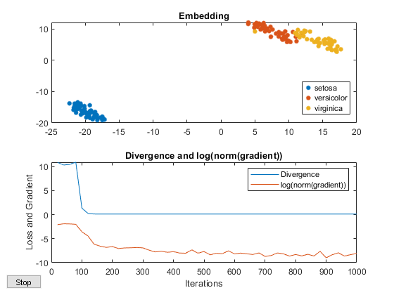
Plot the Fisher iris data, a 4-D data set, in two dimensions using tsne. There is a drop in the Divergence value at iteration 100 because the divergence is scaled by the exaggeration value for earlier iterations. The embedding remains largely unchanged for the last several hundred iterations, so you can save time by clicking the Stop button during the iterations.
load fisheriris
rng default % for reproducibility
opts = statset('OutputFcn',@(optimValues,state) KLLogging(optimValues,state,species));
Y = tsne(meas,'Options',opts,'Algorithm','exact');
