Modify t-SNE Settings
t-SNE is an algorithm for dimensionality reduction that is well-suited to visualizing high-dimensional data. You can use the tsne function to create a set of low-dimensional points (an embedding) and discover natural clusters in the original data. This example shows the effects of modifying the perplexity, exaggeration, and learning rate settings on the low-dimensional embedding of the human activity data set.
Load and Examine Data
Load the humanactivity data set.
load humanactivityThe data set contains observations of 60 predictors for five physical human activities (sitting, standing, walking, running, and dancing), and an activity class label for each observation. For more details on the data set, enter Description at the command line.
The observations are organized by activity class. To better represent a random set of data, shuffle the rows.
n = numel(actid);
rng(0,"twister") % For reproducibility
idx = randsample(n,n);
X = feat(idx,:);
actid = actid(idx);
Associate the activities with the class labels in actid.
activities = ["Sitting" "Standing" "Walking" "Running" "Dancing"]';
activity = activities(actid);
Process Data Using t-SNE
Obtain a two-dimensional embedding of the 60-dimensional data using t-SNE. Use the default settings of Perplexity=30, Exaggeration=4, and LearnRate=500.
rng(0,"twister") % For reproducibility
Y = tsne(X);
figure
numGroups = length(unique(actid));
clr = hsv(numGroups);
gscatter(Y(:,1),Y(:,2),activity,clr)
title("Perplexity: 30, Exaggeration: 4, LearnRate: 500")
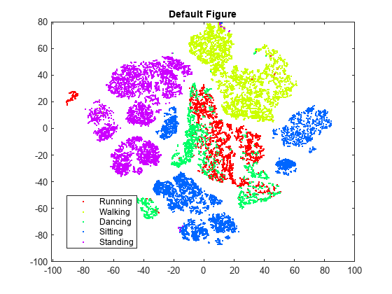
tsne creates an embedding with relatively few data points that seem misplaced. However, the clusters are not well separated.
Perplexity
Try changing the perplexity setting to see the effect on the embedding. First, specify a higher value than the default value of 30, and then specify a lower value.
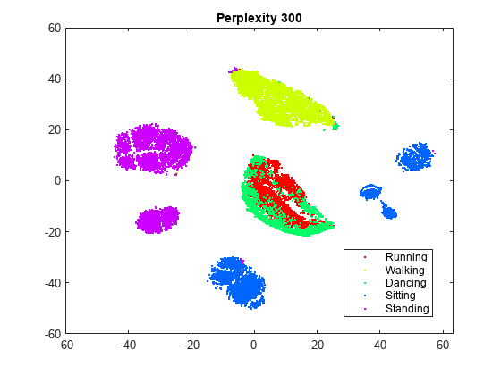
rng(0,"twister") % For fair comparison
Y300 = tsne(X,Perplexity=300);
figure
gscatter(Y300(:,1),Y300(:,2),activity,clr)
title("Perplexity: 300, Exaggeration: 4, LearnRate: 500")
rng(0,"twister") % For fair comparison
Y4 = tsne(X,Perplexity=4);
figure
gscatter(Y4(:,1),Y4(:,2),activity,clr)
title("Perplexity: 4, Exaggeration: 4, LearnRate: 500")
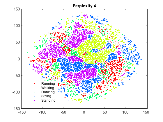
Setting the perplexity to 300 gives an embedding with clusters that are better separated, compared to the original embedding with the default perplexity value of 30. Setting the perplexity to 4 gives an embedding without well-separated clusters. For the remainder of this example, use a perplexity value of 300.
Exaggeration
Try changing the exaggeration setting to see the effect on the embedding. First, specify a higher value than the default value of 4, and then specify a lower value.
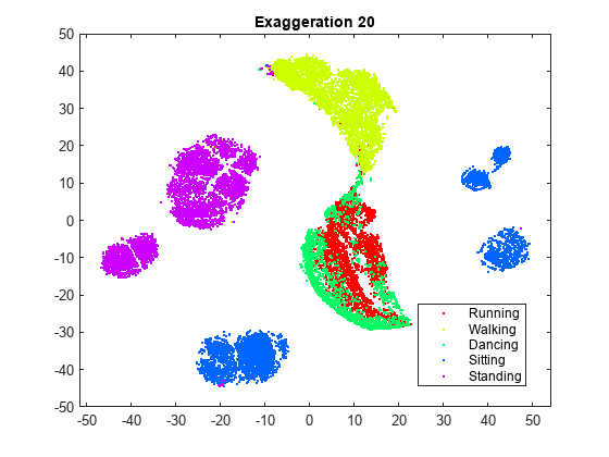
rng(0,"twister") % For fair comparison
YEX20 = tsne(X,Perplexity=300,Exaggeration=75);
figure
gscatter(YEX20(:,1),YEX20(:,2),activity,clr)
title("Perplexity: 300, Exaggeration: 75, LearnRate: 500")
rng(0,"twister") % For fair comparison
YEx15 = tsne(X,Perplexity=300,Exaggeration=1.5);
figure
gscatter(YEx15(:,1),YEx15(:,2),activity,clr)
title("Perplexity: 300, Exaggeration: 1.5, LearnRate: 500")
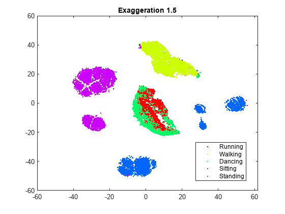
Although the different values for the exaggeration setting have an effect on the embedding, the results do not indicate whether any nondefault value gives a better picture than the default value. In general, a larger exaggeration allows similar points to gather into clusters more effectively and produces more compact clusters. An exaggeration value of 1.5 gives an embedding that is similar to the embedding with the default value of 4. Exaggerating the values in the joint distribution of X makes the values in the joint distribution of Y smaller, which allows the embedded points to move relative to one another more easily.
Learning Rate
Try changing the learning rate setting from its default value of 500 to see the effect on the embedding. First, specify a lower value than the default, and then specify a higher value.
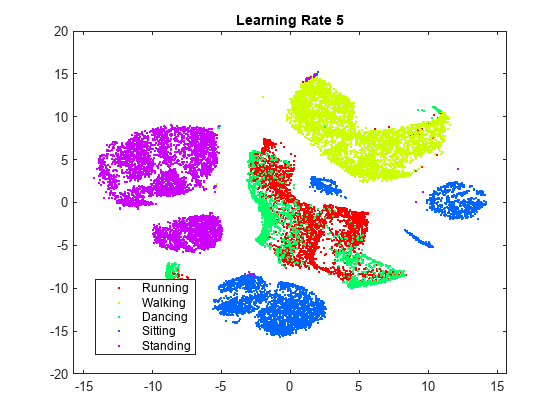
rng(0,"twister") % For fair comparison
YL5 = tsne(X,Perplexity=300,LearnRate=5);
figure
gscatter(YL5(:,1),YL5(:,2),activity,clr)
title("Perplexity: 300, Exaggeration: 4, LearnRate: 5")
rng(0,"twister") % For fair comparison
YL2000 = tsne(X,Perplexity=300,LearnRate=2000);
figure
gscatter(YL2000(:,1),YL2000(:,2),activity,clr)
title("Perplexity: 300, Exaggeration: 4, LearnRate: 2000")
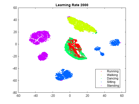
The embedding with a learning rate of 5 has several clusters that split into two or more pieces. This result shows that if the learning rate is too small, the minimization process can get stuck in a bad local minimum. A learning rate of 2000 gives an embedding similar to the one produced with the default learning rate of 500.
Initial Behavior with Various Settings
Large learning rates or exaggeration values can lead to unwanted initial behavior. To see this behavior, set large values of these parameters, and set NumPrint and Verbose to 1 to show all the iterations. Stop after the tenth iteration, because the goal is to look at the initial behavior.
Begin by setting the exaggeration value to 5000.
rng(0,"twister") % For fair comparison
opts = statset(MaxIter=10);
YEX5000 = tsne(X,Perplexity=300,Exaggeration=5000,...
    NumPrint=1,Verbose=1,Options=opts);
|==============================================|
|   ITER   | KL DIVERGENCE   | NORM GRAD USING |
|          | FUN VALUE USING | EXAGGERATED DIST|
|          | EXAGGERATED DIST| OF X            |
|          | OF X            |                 |
|==============================================|
|        1 |    6.388137e+04 |    6.483115e-04 |
|        2 |    6.388775e+04 |    5.267770e-01 |
|        3 |    7.131506e+04 |    5.754291e-02 |
|        4 |    7.234772e+04 |    6.705418e-02 |
|        5 |    7.409144e+04 |    9.278330e-02 |
|        6 |    7.484659e+04 |    1.022587e-01 |
|        7 |    7.445701e+04 |    9.934864e-02 |
|        8 |    7.391345e+04 |    9.633570e-02 |
|        9 |    7.315999e+04 |    1.027610e-01 |
|       10 |    7.265936e+04 |    1.033174e-01 |
The Kullback-Leibler divergence increases during the first few iterations, and then stabilizes. The norm of the gradient jumps sharply at the second iteration, and then fluctuates around 0.1 after the fourth iteration.
To see the final result of the embedding, allow the algorithm to run to completion using the default stopping criteria.
rng(0,"twister") % For fair comparison
YEX5000 = tsne(X,Perplexity=300,Exaggeration=5000);
figure
gscatter(YEX5000(:,1),YEX5000(:,2),activity,clr)
title("Perplexity: 300, Exaggeration: 5000, LearnRate: 500")
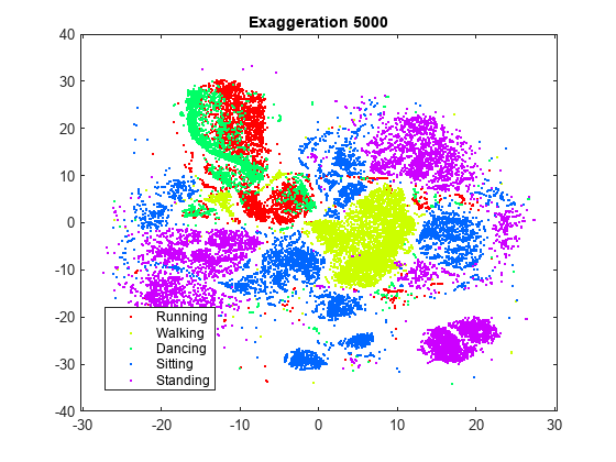
The large exaggeration value of 5000 does not produce well-separated clusters.
Show the initial behavior when the learning rate is 1,000,000.
rng(0,"twister") % For fair comparison
YL1000k = tsne(X,Perplexity=300,LearnRate=1e6,...
    NumPrint=1,Verbose=1,Options=opts);
|==============================================|
|   ITER   | KL DIVERGENCE   | NORM GRAD USING |
|          | FUN VALUE USING | EXAGGERATED DIST|
|          | EXAGGERATED DIST| OF X            |
|          | OF X            |                 |
|==============================================|
|        1 |    2.258150e+01 |    4.412730e-07 |
|        2 |    2.259045e+01 |    4.857725e-04 |
|        3 |    2.945552e+01 |    3.210405e-05 |
|        4 |    2.976546e+01 |    4.337510e-05 |
|        5 |    2.976928e+01 |    4.626810e-05 |
|        6 |    2.969205e+01 |    3.907617e-05 |
|        7 |    2.963695e+01 |    4.943976e-05 |
|        8 |    2.960336e+01 |    4.572338e-05 |
|        9 |    2.956194e+01 |    6.208571e-05 |
|       10 |    2.952132e+01 |    5.253798e-05 |
Again, the Kullback-Leibler divergence increases during the first few iterations and then stabilizes, and the norm of the gradient has an initial large jump and then fluctuates around a constant value.
To see the final result of the embedding, allow the algorithm to run to completion using the default stopping criteria.
rng(0,"twister") % For fair comparison
YL1000k = tsne(X,Perplexity=300,LearnRate=1e6);
figure
gscatter(YL1000k(:,1),YL1000k(:,2),activity,clr)
title("Perplexity: 300, Exaggeration: 4, LearnRate: 1e6")
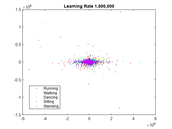
The learning rate is much too large and gives no useful embedding.
Conclusion
tsne with the default settings does a reasonably good job of embedding the initial high-dimensional data into two-dimensional points with well-defined clusters. Increasing the perplexity gives better-separated clusters with this data. The effects of the algorithm settings are difficult to predict, however, and frequently depend on the nature of the data set and its size. The algorithm settings can also affect its speed. For more information, see the tsne reference page.