Main Content

fit

Fit simple model of local interpretable model-agnostic explanations (LIME)

Since R2020b

    Description

    example

    newresults = fit(results,queryPoint,numImportantPredictors) fits a new simple model for the specified query point (queryPoint) by using the specified number of important predictors (numImportantPredictors). The function returns a lime object newresults that contains the new simple model.

    fit uses the simple model options that you specify when you create the lime object results. You can change the options using the name-value pair arguments of the fit function.

    example

    newresults = fit(results,queryPoint,numImportantPredictors,Name,Value) specifies additional options using one or more name-value pair arguments. For example, you can specify 'SimpleModelType','tree' to fit a decision tree model.

    Examples

    collapse all

    Train a regression model and create a lime object that uses a linear simple model. When you create a lime object, if you do not specify a query point and the number of important predictors, then the software generates samples of a synthetic data set but does not fit a simple model. Use the object function fit to fit a simple model for a query point. Then display the coefficients of the fitted linear simple model by using the object function plot.

    Load the carbig data set, which contains measurements of cars made in the 1970s and early 1980s.

    load carbig

    Create a table containing the predictor variables Acceleration, Cylinders, and so on, as well as the response variable MPG.

    tbl = table(Acceleration,Cylinders,Displacement,Horsepower,Model_Year,Weight,MPG);

    Removing missing values in a training set can help reduce memory consumption and speed up training for the fitrkernel function. Remove missing values in tbl.

    tbl = rmmissing(tbl);

    Create a table of predictor variables by removing the response variable from tbl.

    tblX = removevars(tbl,'MPG');

    Train a blackbox model of MPG by using the fitrkernel function.

    rng('default') % For reproducibility
    mdl = fitrkernel(tblX,tbl.MPG,'CategoricalPredictors',[2 5]);

    Create a lime object. Specify a predictor data set because mdl does not contain predictor data.

    results = lime(mdl,tblX)
    results = 
      lime with properties:
    
                 BlackboxModel: [1x1 RegressionKernel]
                  DataLocality: 'global'
         CategoricalPredictors: [2 5]
                          Type: 'regression'
                             X: [392x6 table]
                    QueryPoint: []
        NumImportantPredictors: []
              NumSyntheticData: 5000
                 SyntheticData: [5000x6 table]
                        Fitted: [5000x1 double]
                   SimpleModel: []
           ImportantPredictors: []
                BlackboxFitted: []
             SimpleModelFitted: []


    results contains the generated synthetic data set. The SimpleModel property is empty ([]).

    Fit a linear simple model for the first observation in tblX. Specify the number of important predictors to find as 3.

    queryPoint = tblX(1,:)
    queryPoint=1×6 table
        Acceleration    Cylinders    Displacement    Horsepower    Model_Year    Weight
        ____________    _________    ____________    __________    __________    ______
    
             12             8            307            130            70         3504 
    
    
    results = fit(results,queryPoint,3);

    Plot the lime object results by using the object function plot.

    plot(results)

    The plot displays two predictions for the query point, which correspond to the BlackboxFitted property and the SimpleModelFitted property of results.

    The horizontal bar graph shows the coefficient values of the simple model, sorted by their absolute values. LIME finds Horsepower, Model_Year, and Cylinders as important predictors for the query point.

    Model_Year and Cylinders are categorical predictors that have multiple categories. For a linear simple model, the software creates one less dummy variable than the number of categories for each categorical predictor. The bar graph displays only the most important dummy variable. You can check the coefficients of the other dummy variables using the SimpleModel property of results. Display the sorted coefficient values, including all categorical dummy variables.

    [~,I] = sort(abs(results.SimpleModel.Beta),'descend');
    table(results.SimpleModel.ExpandedPredictorNames(I)',results.SimpleModel.Beta(I), ...
        'VariableNames',{'Expanded Predictor Name','Coefficient'})
    ans=17×2 table
         Expanded Predictor Name      Coefficient
        __________________________    ___________
    
        {'Horsepower'            }    -3.5035e-05
        {'Model_Year (74 vs. 70)'}    -6.1591e-07
        {'Model_Year (80 vs. 70)'}    -3.9803e-07
        {'Model_Year (81 vs. 70)'}     3.4186e-07
        {'Model_Year (82 vs. 70)'}    -2.2331e-07
        {'Cylinders (6 vs. 8)'   }    -1.9807e-07
        {'Model_Year (76 vs. 70)'}      1.816e-07
        {'Cylinders (5 vs. 8)'   }     1.7318e-07
        {'Model_Year (71 vs. 70)'}     1.5694e-07
        {'Model_Year (75 vs. 70)'}     1.5486e-07
        {'Model_Year (77 vs. 70)'}     1.5151e-07
        {'Model_Year (78 vs. 70)'}     1.3864e-07
        {'Model_Year (72 vs. 70)'}     6.8949e-08
        {'Cylinders (4 vs. 8)'   }     6.3098e-08
        {'Model_Year (73 vs. 70)'}     4.9696e-08
        {'Model_Year (79 vs. 70)'}    -2.4822e-08
          ⋮


    Train a classification model and create a lime object that uses a decision tree simple model. Fit multiple models for multiple query points.

    Load the CreditRating_Historical data set. The data set contains customer IDs and their financial ratios, industry labels, and credit ratings.

    tbl = readtable('CreditRating_Historical.dat');

    Create a table of predictor variables by removing the columns of customer IDs and ratings from tbl.

    tblX = removevars(tbl,["ID","Rating"]);

    Train a blackbox model of credit ratings by using the fitcecoc function.

    blackbox = fitcecoc(tblX,tbl.Rating,'CategoricalPredictors','Industry')
    blackbox = 
      ClassificationECOC
               PredictorNames: {'WC_TA'  'RE_TA'  'EBIT_TA'  'MVE_BVTD'  'S_TA'  'Industry'}
                 ResponseName: 'Y'
        CategoricalPredictors: 6
                   ClassNames: {'A'  'AA'  'AAA'  'B'  'BB'  'BBB'  'CCC'}
               ScoreTransform: 'none'
               BinaryLearners: {21x1 cell}
                   CodingName: 'onevsone'


    Create a lime object with the blackbox model.

    rng('default') % For reproducibility
    results = lime(blackbox);

    Find two query points whose true rating values are AAA and B, respectively.

    queryPoint(1,:) = tblX(find(strcmp(tbl.Rating,'AAA'),1),:);
    queryPoint(2,:) = tblX(find(strcmp(tbl.Rating,'B'),1),:)
    queryPoint=2×6 table
        WC_TA    RE_TA    EBIT_TA    MVE_BVTD    S_TA     Industry
        _____    _____    _______    ________    _____    ________
    
        0.121    0.413     0.057      3.647      0.466       12   
        0.019    0.009     0.042      0.257      0.119        1   


    Fit a linear simple model for the first query point. Set the number of important predictors to 4.

    newresults1 = fit(results,queryPoint(1,:),4);

    Plot the LIME results newresults1 for the first query point.

    plot(newresults1)

    Fit a linear decision tree model for the first query point.

    newresults2 = fit(results,queryPoint(1,:),6,'SimpleModelType','tree');
    plot(newresults2)

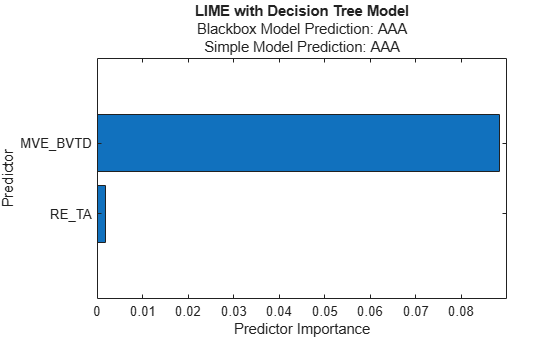
    The simple models in newresults1 and newresults2 both find MVE_BVTD and RE_TA as important predictors.

    Fit a linear simple model for the second query point, and plot the LIME results for the second query point.

    newresults3 = fit(results,queryPoint(2,:),4);
    plot(newresults3)

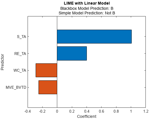
    The prediction from the blackbox model is B, but the prediction from the simple model is not B. When the two predictions are not the same, you can specify a smaller 'KernelWidth' value. The software fits a simple model using weights that are more focused on the samples near the query point. If a query point is an outlier or is located near a decision boundary, then the two prediction values can be different, even if you specify a small 'KernelWidth' value. In such a case, you can change other name-value pair arguments. For example, you can generate a local synthetic data set (specify 'DataLocality' of lime as 'local') for the query point and increase the number of samples ('NumSyntheticData' of lime or fit) in the synthetic data set. You can also use a different distance metric ('Distance' of lime or fit).

    Fit a linear simple model with a small 'KernelWidth' value.

    newresults4 = fit(results,queryPoint(2,:),4,'KernelWidth',0.01);
    plot(newresults4)

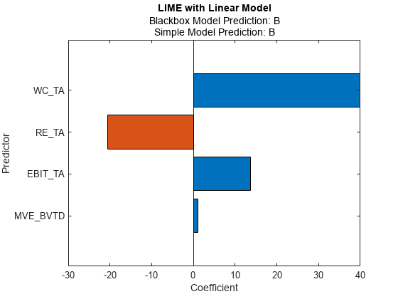
    The credit ratings for the first and second query points are AAA and B, respectively. The simple models in newresults1 and newresults4 both find MVE_BVTD, RE_TA, and WC_TA as important predictors. However, their coefficient values are different. The plots show that these predictors act differently depending on the credit ratings.

    Input Arguments

    collapse all

    LIME results, specified as a lime object.

    Query point around which the fit function fits the simple model, specified as a row vector of numeric values or a single-row table. The queryPoint value must have the same data type and the same number of columns as the predictor data (results.X or results.SyntheticData) in the lime object results.

    queryPoint must not contain missing values.

    Data Types: single | double | table

    Number of important predictors to use in the simple model, specified as a positive integer scalar value.

    • If 'SimpleModelType' is 'linear', then the software selects the specified number of important predictors and fits a linear model of the selected predictors. Note that the software does not use unimportant predictors for fitting the linear model.

    • If 'SimpleModelType' is 'tree', then the software specifies the maximum number of decision splits (or branch nodes) as the number of important predictors so that the fitted decision tree uses at most the specified number of predictors.

    The default value of the numImportantPredictors argument is the NumImportantPredictors property value of the lime object results. If you do not specify the property value when creating results, then the property value is empty ([]) and you must specify this argument.

    Data Types: single | double

    Name-Value Arguments

    Specify optional pairs of arguments as Name1=Value1,...,NameN=ValueN, where Name is the argument name and Value is the corresponding value. Name-value arguments must appear after other arguments, but the order of the pairs does not matter.

    Before R2021a, use commas to separate each name and value, and enclose Name in quotes.

    Example: 'NumSyntheticData',2000,'SimpleModelType','tree' sets the number of samples to generate for the synthetic data set to 2000 and specifies the simple model type as a decision tree.

    Since R2023b

    Relative tolerance on the linear coefficients and the bias term (intercept) for the linear simple model, specified as a nonnegative scalar.

    This argument is valid only when the SimpleModelType value is "linear".

    Let Bt=[βtbt], that is, the vector of the coefficients and the bias term at fitting step t. If BtBt1Bt2<BetaTolerance, then the fitting process for the linear simple model terminates.

    Example: "BetaTolerance",1e-8

    Data Types: single | double

    Covariance matrix for the Mahalanobis distance metric, specified as the comma-separated pair consisting of 'Cov' and a K-by-K positive definite matrix, where K is the number of predictors.

    This argument is valid only if 'Distance' is 'mahalanobis'.

    The default value is the 'Cov' value that you specify when creating the lime object results. The default 'Cov' value of lime is cov(PD,'omitrows'), where PD is the predictor data or synthetic predictor data. If you do not specify the 'Cov' value, then the software uses different covariance matrices when computing the distances for both the predictor data and the synthetic predictor data.

    Example: 'Cov',eye(3)

    Data Types: single | double

    Distance metric, specified as the comma-separated pair consisting of 'Distance' and a character vector, string scalar, or function handle.

    • If the predictor data includes only continuous variables, then fit supports these distance metrics.

      ValueDescription
      'euclidean'

      Euclidean distance.

      'seuclidean'

      Standardized Euclidean distance. Each coordinate difference between observations is scaled by dividing by the corresponding element of the standard deviation, S = std(PD,'omitnan'), where PD is the predictor data or synthetic predictor data. To specify different scaling, use the 'Scale' name-value argument.

      'mahalanobis'

      Mahalanobis distance using the sample covariance of PD, C = cov(PD,'omitrows'). To change the value of the covariance matrix, use the 'Cov' name-value argument.

      'cityblock'

      City block distance.

      'minkowski'

      Minkowski distance. The default exponent is 2. To specify a different exponent, use the 'P' name-value argument.

      'chebychev'

      Chebychev distance (maximum coordinate difference).

      'cosine'

      One minus the cosine of the included angle between points (treated as vectors).

      'correlation'

      One minus the sample correlation between points (treated as sequences of values).

      'spearman'

      One minus the sample Spearman's rank correlation between observations (treated as sequences of values).

      @distfun

      Custom distance function handle. A distance function has the form

      function D2 = distfun(ZI,ZJ)
      % calculation of distance
      ...
      where

      • ZI is a 1-by-t vector containing a single observation.

      • ZJ is an s-by-t matrix containing multiple observations. distfun must accept a matrix ZJ with an arbitrary number of observations.

      • D2 is an s-by-1 vector of distances, and D2(k) is the distance between observations ZI and ZJ(k,:).

      If your data is not sparse, you can generally compute distance more quickly by using a built-in distance metric instead of a function handle.

    • If the predictor data includes both continuous and categorical variables, then fit supports these distance metrics.

      ValueDescription
      'goodall3'

      Modified Goodall distance

      'ofd'

      Occurrence frequency distance

    For definitions, see Distance Metrics.

    The default value is the 'Distance' value that you specify when creating the lime object results. The default 'Distance' value of lime is 'euclidean' if the predictor data includes only continuous variables, or 'goodall3' if the predictor data includes both continuous and categorical variables.

    Example: 'Distance','ofd'

    Data Types: char | string | function_handle

    Kernel width of the squared exponential (or Gaussian) kernel function, specified as the comma-separated pair consisting of 'KernelWidth' and a numeric scalar value.

    The fit function computes distances between the query point and the samples in the synthetic predictor data set, and then converts the distances to weights by using the squared exponential kernel function. If you lower the 'KernelWidth' value, then fit uses weights that are more focused on the samples near the query point. For details, see LIME.

    The default value is the 'KernelWidth' value that you specify when creating the lime object results. The default 'KernelWidth' value of lime is 0.75.

    Example: 'KernelWidth',0.5

    Data Types: single | double

    Number of neighbors of the query point, specified as the comma-separated pair consisting of 'NumNeighbors' and a positive integer scalar value. This argument is valid only when the DataLocality property of results is 'local'.

    The fit function estimates the distribution parameters of the predictor data using the specified number of nearest neighbors of the query point. Then the function generates synthetic predictor data using the estimated distribution.

    If you specify a value larger than the number of observations in the predictor data set (results.X) in the lime object results, then fit uses all observations.

    The default value is the 'NumNeighbors' value that you specify when creating the lime object results. The default 'NumNeighbors' value of lime is 1500.

    Example: 'NumNeighbors',2000

    Data Types: single | double

    Number of samples to generate for the synthetic data set, specified as the comma-separated pair consisting of 'NumSyntheticData' and a positive integer scalar value.

    The default value is the NumSyntheticData property value of the lime object results. If you provide a custom synthetic data set when creating results, then the property value is the number of samples in the data set. Otherwise, the 'NumSyntheticData' value that you specify when creating results sets the property. The default 'NumSyntheticData' value of lime is 5000.

    Example: 'NumSyntheticData',2500

    Data Types: single | double

    Exponent for the Minkowski distance metric, specified as the comma-separated pair consisting of 'P' and a positive scalar.

    This argument is valid only if 'Distance' is 'minkowski'.

    The default value is the 'P' value that you specify when creating the lime object results. The default 'P' value of lime is 2.

    Example: 'P',3

    Data Types: single | double

    Scale parameter value for the standardized Euclidean distance metric, specified as the comma-separated pair consisting of 'Scale' and a nonnegative numeric vector of length K, where K is the number of predictors.

    This argument is valid only if 'Distance' is 'seuclidean'.

    The default value is the 'Scale' value that you specify when creating the lime object results. The default 'Scale' value of lime is std(PD,'omitnan'), where PD is the predictor data or synthetic predictor data. If you do not specify the 'Scale' value, then the software uses different scale parameters when computing the distances for both the predictor data and the synthetic predictor data.

    Example: 'Scale',quantile(X,0.75) - quantile(X,0.25)

    Data Types: single | double

    Type of the simple model, specified as the comma-separated pair consisting of 'SimpleModelType' and 'linear' or 'tree'.

    • 'linear' — The software fits a linear model by using fitrlinear for regression or fitclinear for classification.

    • 'tree' — The software fits a decision tree model by using fitrtree for regression or fitctree for classification.

    The default value is the 'SimpleModelType' value that you specify when creating the lime object results. The default 'SimpleModelType' value of lime is 'linear'.

    Example: 'SimpleModelType','tree'

    Data Types: char | string

    Output Arguments

    collapse all

    LIME results, returned as a lime object. newresults contains the new simple model.

    To overwrite the input argument results, assign the output of fit to results:

    results = fit(results,queryPoint,numImportantPredictors);

    More About

    collapse all

    Distance Metrics

    A distance metric is a function that defines a distance between two observations. fit supports various distance metrics for continuous variables and a mix of continuous and categorical variables.

    • Distance metrics for continuous variables

      Given an mx-by-n data matrix X, which is treated as mx (1-by-n) row vectors x1, x2, ..., xmx, and an my-by-n data matrix Y, which is treated as my (1-by-n) row vectors y1, y2, ...,ymy, the various distances between the vector xs and yt are defined as follows:

      • Euclidean distance

        dst2=(xsyt)(xsyt).

        The Euclidean distance is a special case of the Minkowski distance, where p = 2.

        Specify Euclidean distance by setting the Distance parameter to 'euclidean'.

      • Standardized Euclidean distance

        dst2=(xsyt)V1(xsyt),

        where V is the n-by-n diagonal matrix whose jth diagonal element is (S(j))2, where S is a vector of scaling factors for each dimension.

        Specify standardized Euclidean distance by setting the Distance parameter to 'seuclidean'.

      • Mahalanobis distance

        dst2=(xsyt)C1(xsyt),

        where C is the covariance matrix.

        Specify Mahalanobis distance by setting the Distance parameter to 'mahalanobis'.

      • City block distance

        dst=j=1n|xsjytj|.

        The city block distance is a special case of the Minkowski distance, where p = 1.

        Specify city block distance by setting the Distance parameter to 'cityblock'.

      • Minkowski distance

        dst=j=1n|xsjytj|pp.

        For the special case of p = 1, the Minkowski distance gives the city block distance. For the special case of p = 2, the Minkowski distance gives the Euclidean distance. For the special case of p = ∞, the Minkowski distance gives the Chebychev distance.

        Specify Minkowski distance by setting the Distance parameter to 'minkowski'.

      • Chebychev distance

        dst=maxj{|xsjytj|}.

        The Chebychev distance is a special case of the Minkowski distance, where p = ∞.

        Specify Chebychev distance by setting the Distance parameter to 'chebychev'.

      • Cosine distance

        dst=(1xsyt(xsxs)(ytyt)).

        Specify cosine distance by setting the Distance parameter to 'cosine'.

      • Correlation distance

        dst=1(xsx¯s)(yty¯t)(xsx¯s)(xsx¯s)(yty¯t)(yty¯t),

        where

        x¯s=1njxsj

        and

        y¯t=1njytj.

        Specify correlation distance by setting the Distance parameter to 'correlation'.

      • Spearman distance is one minus the sample Spearman's rank correlation between observations (treated as sequences of values):

        dst=1(rsr¯s)(rtr¯t)(rsr¯s)(rsr¯s)(rtr¯t)(rtr¯t),

        where

        • rsj is the rank of xsj taken over x1j, x2j, ...xmx,j, as computed by tiedrank.

        • rtj is the rank of ytj taken over y1j, y2j, ...ymy,j, as computed by tiedrank.

        • rs and rt are the coordinate-wise rank vectors of xs and yt, that is, rs = (rs1, rs2, ... rsn) and rt = (rt1, rt2, ... rtn).

        • r¯s=1njrsj=(n+1)2.

        • r¯t=1njrtj=(n+1)2.

        Specify Spearman distance by setting the Distance parameter to 'spearman'.

    • Distance metrics for a mix of continuous and categorical variables

      • Modified Goodall distance

        This distance is a variant of the Goodall distance, which assigns a small distance if the matching values are infrequent regardless of the frequencies of the other values. For mismatches, the distance contribution of the predictor is 1/(number of variables).

        Specify modified Goodall distance by setting the Distance parameter to 'goodall3'.

      • Occurrence frequency distance

        For a match, the occurrence frequency distance assigns zero distance. For a mismatch, the occurrence frequency distance assigns a higher distance on a less frequent value and a lower distance on a more frequent value.

        Specify occurrence frequency distance by setting the Distance parameter to 'ofd'.

    Algorithms

    collapse all

    LIME

    To explain a prediction of a machine learning model using LIME [1], the software generates a synthetic data set and fits a simple interpretable model to the synthetic data set by using lime and fit, as described in steps 1–5.

    • If you specify the queryPoint and numImportantPredictors values of lime, then the lime function performs all steps.

    • If you do not specify queryPoint and numImportantPredictors and specify 'DataLocality' as 'global' (default), then the lime function generates a synthetic data set (steps 1–2), and the fit function fits a simple model (steps 3–5).

    • If you do not specify queryPoint and numImportantPredictors and specify 'DataLocality' as 'local', then the fit function performs all steps.

    The lime and fit functions perform these steps:

    1. Generate a synthetic predictor data set Xs using a multivariate normal distribution for continuous variables and a multinomial distribution for each categorical variable. You can specify the number of samples to generate by using the 'NumSyntheticData' name-value argument.

      • If 'DataLocality' is 'global' (default), then the software estimates the distribution parameters from the whole predictor data set (X or predictor data in blackbox).

      • If 'DataLocality' is 'local', then the software estimates the distribution parameters using the k-nearest neighbors of the query point, where k is the 'NumNeighbors' value. You can specify a distance metric to find the nearest neighbors by using the 'Distance' name-value argument.

      The software ignores missing values in the predictor data set when estimating the distribution parameters.

      Alternatively, you can provide a pregenerated, custom synthetic predictor data set by using the customSyntheticData input argument of lime.

    2. Compute the predictions Ys for the synthetic data set Xs. The predictions are predicted responses for regression or classified labels for classification. The software uses the predict function of the blackbox model to compute the predictions. If you specify blackbox as a function handle, then the software computes the predictions by using the function handle.

    3. Compute the distances d between the query point and the samples in the synthetic predictor data set using the distance metric specified by 'Distance'.

    4. Compute the weight values wq of the samples in the synthetic predictor data set with respect to the query point q using the squared exponential (or Gaussian) kernel function

      wq(xs)=exp(12(d(xs,q)pσ)2).

      • xs is a sample in the synthetic predictor data set Xs.

      • d(xs,q) is the distance between the sample xs and the query point q.

      • p is the number of predictors in Xs.

      • σ is the kernel width, which you can specify by using the 'KernelWidth' name-value argument. The default 'KernelWidth' value is 0.75.

      The weight value at the query point is 1, and then it converges to zero as the distance value increases. The 'KernelWidth' value controls how fast the weight value converges to zero. The lower the 'KernelWidth' value, the faster the weight value converges to zero. Therefore, the algorithm gives more weight to samples near the query point. Because this algorithm uses such weight values, the selected important predictors and fitted simple model effectively explain the predictions for the synthetic data locally, around the query point.

    5. Fit a simple model.

      • If 'SimpleModelType' is 'linear' (default), then the software selects important predictors and fits a linear model of the selected important predictors.

        • Select n important predictors (X˜s) by using the group orthogonal matching pursuit (OMP) algorithm [2][3], where n is the numImportantPredictors value. This algorithm uses the synthetic predictor data set (Xs), predictions (Ys), and weight values (wq).

          Note that the software does not select unimportant predictors (with estimated 0 coefficients), so the number of selected important predictors can be less than n.

        • Fit a linear model of the selected important predictors (X˜s) to the predictions (Ys) using the weight values (wq). The software uses fitrlinear for regression or fitclinear for classification. For a multiclass model, the software uses the one-versus-all scheme to construct a binary classification problem. The positive class is the predicted class for the query point from the blackbox model, and the negative class refers to the other classes.

      • If 'SimpleModelType' is 'tree', then the software fits a decision tree model by using fitrtree for regression or fitctree for classification. The software specifies the maximum number of decision splits (or branch nodes) as the number of important predictors so that the fitted decision tree uses at most the specified number of predictors.

    References

    [1] Ribeiro, Marco Tulio, S. Singh, and C. Guestrin. "'Why Should I Trust You?': Explaining the Predictions of Any Classifier." In Proceedings of the 22nd ACM SIGKDD International Conference on Knowledge Discovery and Data Mining, 1135–44. San Francisco, California: ACM, 2016.

    [2] Świrszcz, Grzegorz, Naoki Abe, and Aurélie C. Lozano. "Grouped Orthogonal Matching Pursuit for Variable Selection and Prediction." Advances in Neural Information Processing Systems (2009): 1150–58.

    [3] Lozano, Aurélie C., Grzegorz Świrszcz, and Naoki Abe. "Group Orthogonal Matching Pursuit for Logistic Regression." Proceedings of the Fourteenth International Conference on Artificial Intelligence and Statistics (2011): 452–60.

    Version History

    Introduced in R2020b

    expand all