plotResiduals
Syntax
Description
plotResiduals( creates a histogram plot
of the censored linear regression model (mdl)mdl) residuals.
plotResiduals(
specifies additional options using one or more name-value arguments. For example, you can
specify the residual type and the graphical properties of residual data points.mdl,plottype,Name=Value)
plotResiduals( creates
the plot in the axes specified by ax,___)ax instead of the current axes,
using any of the input argument combinations in the previous syntaxes.
h = plotResiduals(___)h to modify
the properties of a specific line or patch after you create the plot. For a list of
properties, see Line Properties and Patch Properties.
Examples
Load the readmissiontimes data set, and fit a censored linear regression model of the readmission time as a function of patient age, weight, and smoking status.
load readmissiontimes
tbl = table(Age,Weight,Smoker,Censored,ReadmissionTime);
mdl = fitlmcens(tbl,Censoring="Censored",CategoricalVars="Smoker");
Create a histogram of the raw residuals.
plotResiduals(mdl)
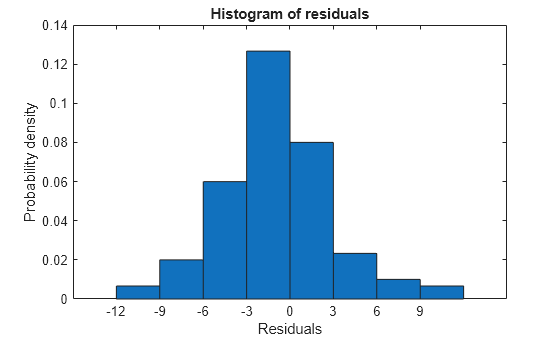
The area of each bar is the relative number of observations. The sum of the bar areas is equal to 1. The histogram indicates that the residuals are approximately normally distributed.
Load the censoreddata sample data.
load censoreddata.matThe matrix X contains data for three predictors, and the matrix yint contains bounds for a censored response variable.
Fit a linear regression model to the censored data in X and yint.
mdl = fitlmcens(X,yint);
Display a probability plot of the standardized residuals.
plotResiduals(mdl,"probability",ResidualType="standardized")
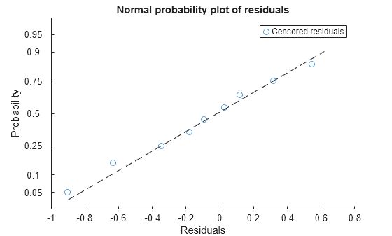
The plot shows that the standardized residuals have a normal distribution (approximately).
Input Arguments
Name-Value Arguments
Specify optional pairs of arguments as
Name1=Value1,...,NameN=ValueN, where Name is
the argument name and Value is the corresponding value.
Name-value arguments must appear after other arguments, but the order of the
pairs does not matter.
Example: plotResiduals(mdl,"probability",Residuals="standardized",Color="m")
specifies magenta markers and standardized residuals for a probability plot of the residuals
in mdl.
Note
The graphical properties listed here are only a subset. For a complete list, see Line Properties for lines and Patch Properties for histograms. The specified properties apply to the appearance of residual data points or the appearance of the histogram.
Line color, specified an RGB triplet, hexadecimal color code, color name, or short name for one of the color options listed in the following table.
The Color name-value argument also determines marker outline color and
marker fill color if MarkerEdgeColor is
"auto" (default) and MarkerFaceColor is
"auto".
For a custom color, specify an RGB triplet or a hexadecimal color code.
An RGB triplet is a three-element row vector whose elements specify the intensities of the red, green, and blue components of the color. The intensities must be in the range
[0,1], for example,[0.4 0.6 0.7].A hexadecimal color code is a string scalar or character vector that starts with a hash symbol (
#) followed by three or six hexadecimal digits, which can range from0toF. The values are not case sensitive. Therefore, the color codes"#FF8800","#ff8800","#F80", and"#f80"are equivalent.
Alternatively, you can specify some common colors by name. This table lists the named color options, the equivalent RGB triplets, and the hexadecimal color codes.
| Color Name | Short Name | RGB Triplet | Hexadecimal Color Code | Appearance |
|---|---|---|---|---|
"red" | "r" | [1 0 0] | "#FF0000" |
|
"green" | "g" | [0 1 0] | "#00FF00" |
|
"blue" | "b" | [0 0 1] | "#0000FF" |
|
"cyan"
| "c" | [0 1 1] | "#00FFFF" |
|
"magenta" | "m" | [1 0 1] | "#FF00FF" |
|
"yellow" | "y" | [1 1 0] | "#FFFF00" |
|
"black" | "k" | [0 0 0] | "#000000" |
|
"white" | "w" | [1 1 1] | "#FFFFFF" |
|
"none" | Not applicable | Not applicable | Not applicable | No color |
This table lists the default color palettes for plots in the light and dark themes.
| Palette | Palette Colors |
|---|---|
Before R2025a: Most plots use these colors by default. |
|
|
|
You can get the RGB triplets and hexadecimal color codes for these palettes using the orderedcolors and rgb2hex functions. For example, get the RGB triplets for the "gem" palette and convert them to hexadecimal color codes.
RGB = orderedcolors("gem");
H = rgb2hex(RGB);
Before R2023b: Get the RGB triplets using RGB =
get(groot,"FactoryAxesColorOrder").
Before R2024a: Get the hexadecimal color codes using H =
compose("#%02X%02X%02X",round(RGB*255)).
Example: Color="blue"
Data Types: single | double | string | char
Line width, specified as a positive value in points. If the line has markers, then the line width also affects the marker edges.
Example: LineWidth=0.75
Data Types: single | double
Marker symbol, specified as one of the values in this table.
| Marker | Description | Resulting Marker |
|---|---|---|
"o" | Circle |
|
"+" | Plus sign |
|
"*" | Asterisk |
|
"." | Point |
|
"x" | Cross |
|
"_" | Horizontal line |
|
"|" | Vertical line |
|
"square" | Square |
|
"diamond" | Diamond |
|
"^" | Upward-pointing triangle |
|
"v" | Downward-pointing triangle |
|
">" | Right-pointing triangle |
|
"<" | Left-pointing triangle |
|
"pentagram" | Pentagram |
|
"hexagram" | Hexagram |
|
"none" | No markers | Not applicable |
Example: Marker="+"
Data Types: string | char
Marker outline color, specified an RGB triplet, hexadecimal color code, color
name, or short name for one of the color options listed in the
Color name-value argument.
The default value "auto" uses the same color specified by using
the Color name-value argument. You can also specify
"none" for no color.
Example: MarkerEdgeColor="blue"
Data Types: single | double | string | char
Marker fill color, specified as an RGB triplet, hexadecimal color code, color name, or short
name for one of the color options listed in the Color
name-value argument. The default value "none" specifies no
color.
The "auto" value uses the same color specified by using the
Color name-value argument.
Example: MarkerFaceColor="blue"
Data Types: single | double | string | char
Marker size, specified as a positive value in points.
Example: MarkerSize=2
Data Types: single | double
Output Arguments
Alternative Functionality
A CensoredLinearModel
object provides multiple plotting functions. After fitting a model, use plotPartialDependence to understand the effect of a particular predictor. Use
plotSlice to plot
slices through the prediction surface.
Version History
Introduced in R2025a