plotSlice

Plot of slices through fitted censored linear regression surface

Since R2025a

Syntax

plotSlice(mdl)

plotSlice(mdl,Xnew)

plotSlice(fig,___)

Description

plotSlice(mdl) creates a figure containing one or more plots, each representing a slice through the regression surface predicted by mdl. Each plot shows the fitted response values as a function of a single predictor variable, with the other predictor variables held constant.

plotSlice also displays the 95% confidence bounds for the response values. You can specify the type of confidence bounds, and select which predictors to use for each slice plot. For more information, see Tips.

plotSlice(mdl,Xnew) uses the predictor data in Xnew to create the figure.

plotSlice(fig,___) plots into the figure fig instead of the current figure (gcf) using any of the input argument combinations in the previous syntaxes.

Examples

Plot Responses for Censored Linear Regression Model

Load the readmissiontimes sample data.

load readmissiontimes

The variables Age, Weight, Smoker, and ReadmissionTime contain data for patient age, weight, smoking status, and time of readmission. The Censored variable contains censoring information for ReadmissionTime.

Save Age, Weight, Smoker, and ReadmissionTime in a table, and fit a censored linear regression model to the data.

tbl = table(Age,Weight,Smoker,ReadmissionTime);
mdl = fitlmcens(tbl,Censoring=Censored,CategoricalVars="Smoker");

mdl is a CensoredLinearModel object that contains the results of fitting a linear model to the censored data.

Create a slice plot for mdl.

plotSlice(mdl)

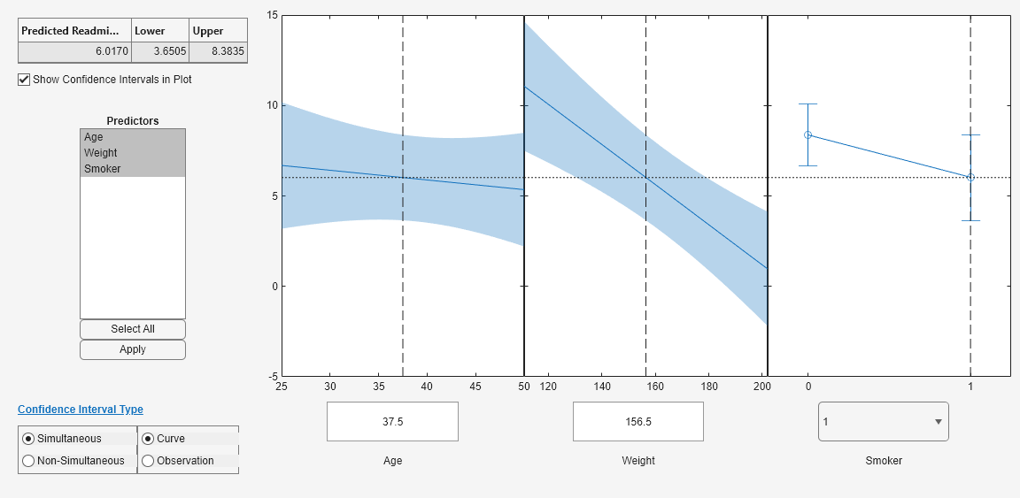
Each plot shows ReadmissionTime as a function of a single predictor variable; Age in the plot on the left, Weight in the plot in the center, and Smoker in the plot on the right. The predictor is fixed at the value shown in the x-axis of each plot. The 95% confidence intervals for the continuous predictors Age and Weight are represented by a blue shaded region. The 95% confidence intervals for the categorical predictor Smoker are represented by error bars. The dashed lines indicate a selected point, and the table to the left of the plots shows the response value and confidence bounds for the selected point. You can select a different point by changing the predictor values in the x-axis labels or by dragging the dashed lines to a different location.

Change the value of Weight to 200.

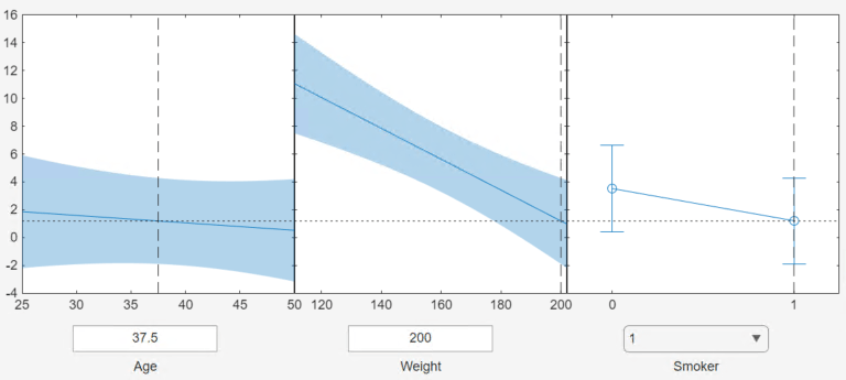
The right plot shows that the value for ReadmissionTime is smaller for patients with a weight of 200, relative to patients with a weight of 156.5, across all values for Age and Smoker.

Specify Predictor Data for Slice Plot

Load the readmissiontimes sample data.

load readmissiontimes

The variables Age, Weight, Smoker, and ReadmissionTime contain data for patient age, weight, smoking status, and time of readmission. The Censored variable contains censoring information for ReadmissionTime.

Save Age, Weight, Smoker, and ReadmissionTime in a table, and fit a censored linear regression model to the data.

tbl = table(Age,Weight,Smoker,ReadmissionTime);
mdl = fitlmcens(tbl,Censoring=Censored,CategoricalVars="Smoker");

mdl is a CensoredLinearModel object that contains the results of fitting a linear model to the censored data.

Generate new predictor data for patient age, weight, and smoking status.

Age_New = 25:35;
Weight_New = 100:10:200;
Smoker_New = binornd(1,0.5,11,1);
Xnew = [Age_New',Weight_New',Smoker_New];

Create a slice plot for mdl using the new predictor data.

plotSlice(mdl,Xnew)

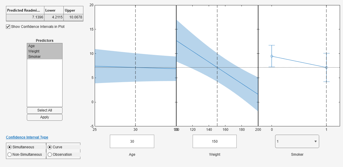
The left plot shows ReadmissionTime as a function of Age with Weight fixed at 150 and Smoker fixed at 1. The center plot shows ReadmissionTime as a function of Weight with Age fixed at 30 and Smoker fixed at 1. The right plot shows ReadmissionTime as a function of Smoker with Age fixed at 30 and Weight fixed at 150.

Plot Single Predictor

Load the readmissiontimes sample data.

load readmissiontimes

The variables Age and ReadmissionTime contain data for patient age and time of readmission. The Censored variable contains censoring information for ReadmissionTime.

Save Age and ReadmissionTime in a table, and fit a censored linear regression model to the data.

tbl = table(Age,ReadmissionTime);
mdl = fitlmcens(tbl,Censoring=Censored);

mdl is a CensoredLinearModel object that contains the results of fitting a linear model to the censored data.

Create a slice plot for mdl.

plotSlice(mdl)

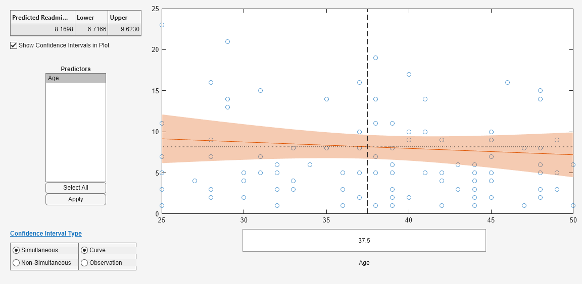
Because mdl has only one predictor, the slice plot displays a single set of axes containing a scatter plot of the training data. The regression line for mdl is shown in red together with a shaded region representing the 95% confidence intervals. The Confidence Interval Type options indicate that the confidence interval is simultaneous and pertains to the fitted responses. For more information, see Tips.

Input Arguments

mdl — Censored linear regression model

CensoredLinearModel object | CompactCensoredLinearModel object

Censored linear regression model, specified as a CensoredLinearModel object created using fitlmcens, or a CompactCensoredLinearModel object created using fitlmcens and compact.

Xnew — New predictor input values

table | numeric matrix

New predictor input values, specified as a table or numeric matrix. If Xnew is a table, its columns must have the same names as the predictors in mdl.VariableNames. If Xnew is a matrix, its columns must correspond to the predictors in mdl.VariableNames. Xnew cannot contain categorical predictor values not used during training.

Data Types: single | double | table

fig — Target figure

Figure object

Target figure, specified as a Figure object. You must create fig using the uifigure function. If you do not specify fig, then plotSlice creates a new figure.

Tips

• Use the Confidence Interval Type options in the figure window to specify the type of confidence bounds. You can specify simultaneous or nonsimultaneous, and curve or observation.

  • Simultaneous or Non-Simultaneous

    • Simultaneous (default) — plotSlice computes confidence bounds for the curve of the response values using Scheffé's method. The range between the upper and lower confidence bounds contains the curve consisting of true response values with 95% confidence.

    • Non-Simultaneous — plotSlice computes confidence bounds for the response value at each observation. The confidence interval for a response value at a specific predictor value contains the true response value with 95% confidence.

    With simultaneous bounds, the entire curve of true response values is within the bounds at high confidence. By contrast, non-simultaneous bounds require only the response value at a single predictor value to be within the bounds at high confidence. Therefore, simultaneous bounds are wider than non-simultaneous bounds.

    If you do not want the plot to display confidence bounds, you can clear the Show Confidence Intervals in Plot box.

  • Curve or Observation

    A regression model for the predictor variables X and the response variable y has the form

    y = f(X) + ε,

    where f is a function of X and ε is a random noise term.

    • Curve (default) — plotSlice predicts confidence bounds for the fitted responses f(X).

    • Observation — plotSlice predicts confidence bounds for the response observations y.

    The bounds for y are wider than the bounds for f(X) because of the additional variability of the noise term.

• Use the Predictors options to select which predictors to use for each slice plot. If the regression model mdl includes more than eight predictors, plotSlice creates plots for the first five predictors by default.

Alternative Functionality

• Use predict to return the predicted response values and confidence bounds. You can also specify the confidence level for confidence bounds by using the Alpha name-value argument of the predict function. Note that predict finds nonsimultaneous bounds by default, whereas plotSlice finds simultaneous bounds by default.

• A CensoredLinearModel object provides multiple plotting functions.

  • When verifying a model, use plotResiduals to analyze the residuals of the model.

  • After fitting a model, use plotPartialDependence to understand the effect of a particular predictor.

Version History

Introduced in R2025a