Batch Compute Steady-State Operating Points for Parameter Variation
Block parameters configure a Simulink® model in several ways. For example, you can use block parameters to specify various coefficients or controller sample times. You can also use a discrete parameter, like the control input to a Multiport Switch block, to control the data path within a model. Varying the value of a parameter helps you understand its impact on the model behavior. Also, you can vary the parameters of a plant model in a control system to study the robustness of the controller to plant variations.
When trimming a model using findop, you can specify a set
of parameter values for which to trim the model. The full set of values is called
a parameter grid or parameter
samples. findop computes an operating point
for each value combination in the parameter grid. You can vary multiple
parameters, thus extending the parameter grid dimension.
Which Parameters Can Be Sampled?
You can vary any model parameter with a value given by a variable in the
model workspace, the MATLAB® workspace, or a data dictionary. In cases where the varying
parameters are all tunable, findop requires only one model
compilation to find operating points for varying parameter values. This
efficiency is especially advantageous for models that are expensive to
compile repeatedly.
Vary Single Parameter
To vary the value of a single parameter for batch trimming with
findop, specify the parameter grid as a structure
having two fields. The Name field contains the name of
the workspace variable that specifies the parameter. The
Value field contains a vector of values for that
parameter to take during trimming.
For example, the Watertank model has three
parameters defined as MATLAB workspace variables, a, b,
and A. The following commands specify a parameter
grid for the single parameter for A.
param.Name = 'A';
param.Value = Avals;
Here, Avals is an array specifying the sample
values for A.
The following table lists some common ways of specifying parameter samples.
| Parameter Sample-Space Type | How to Specify the Parameter Samples |
|---|---|
| Evenly spaced values across a given range | param.Value = [Amin:1:Amax] |
| Linearly spaced values across a given range | param.Value = linspace(Amin,Amax,N) |
| Logarithmically spaced values across a given range | param.Value = logspace(Amin,Amax,N) |
| Random values | param.Value = rand(1,N) |
| Custom vector | param.Value = [value1,value2,...,valueN] |
If the variable used by the model is not a scalar variable,
specify the parameter name as an expression that resolves to a numeric
scalar value. For example, suppose that Kpid is
a vector of PID gains. The first entry in that vector, Kpid,
is used as a gain value in a block in your model. Use the following
commands to vary that gain using the values given in a vector Kpvals:
param.Name = 'Kpid(1)';
param.Value = Kpvals;
After you create the structure param, pass it to
findop as the param input
argument.
Multidimensional Parameter Grids
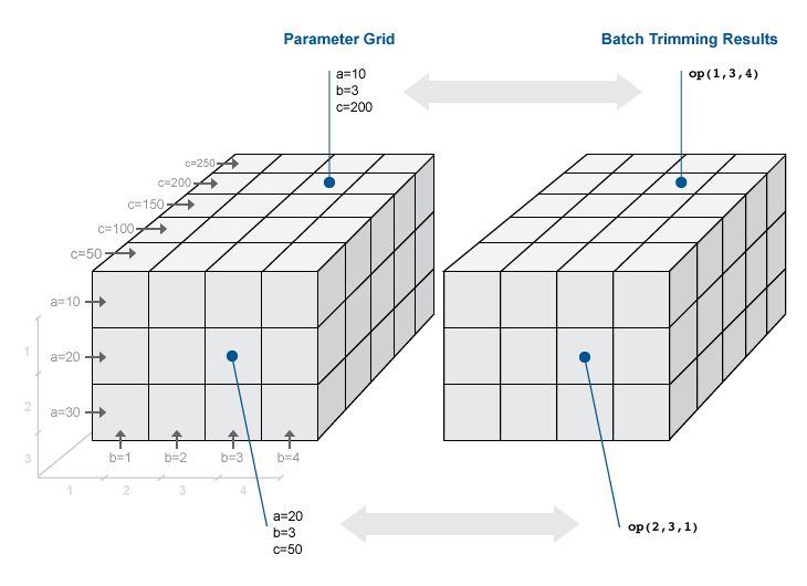
When you vary more than one parameter at a time, you generate parameter grids of higher dimension. For example, varying two parameters yields a parameter matrix, and varying three parameters yields a 3-D parameter grid. Consider the following parameter grid used for batch trimming:

Here, you vary the values of three parameters, a,
b, and c. The samples form a
3-by-4-by-5 grid. op is an array with same dimensions
that contains corresponding trimmed operating point objects.
Vary Multiple Parameters
To vary the value of multiple parameters for batch trimming with
findop, specify parameter samples as a structure
array. The structure has an entry for each parameter whose value you vary.
The structure for each parameter is the same as described in Vary Single Parameter. You can
specify the Value field for a parameter as an array of
any dimension. However, the size of the Value field must
match for all parameters. Corresponding array entries for all the
parameters, also referred to as a parameter grid
points, must map to a specified parameter combination.
When the software trims the model, it computes an operating point for each
grid point.
Specify Full Grid
Suppose that your model has two parameters whose values you want to vary, a and b:
You want to trim the model for every combination of a and b, also referred to as a full grid:
Create a rectangular parameter grid using ndgrid.
a1 = 1;
a2 = 2;
a = [a1 a2];

b1 = 3;
b2 = 4;
b = [b1 b2];

[A,B] = ndgrid(a,b)
A =

     1     1
     2     2

B =

     3     4
     3     4
Create the structure array, params, that
specifies the parameter grid.
params(1).Name = 'a';
params(1).Value = A;

params(2).Name = 'b';
params(2).Value = B;
In general, to specify a full grid for N parameters,
use ndgrid to obtain N grid
arrays.
[P1,...,PN] = ndgrid(p1,...,pN);
Here, p1,...,pN are
the parameter sample vectors.
Create a 1 x N structure array.
params(1).Name = 'p1';
params(1).Value = P1;
...
params(N).Name = 'pN';
params(N).Value = PN;
Specify Subset of Full Grid
If your model is complex or you vary the value of many parameters, trimming the model for the full grid can become expensive. In this case, you can specify a subset of the full grid using a table-like approach. Using the example in Specify Full Grid, suppose that you want to trim the model for the following combinations of a and b:
Create the structure array, params, that
specifies this parameter grid.
A = [a1 a1];
params(1).Name = 'a';
params(1).Value = A;

B = [b1 b2];
params(2).Name = 'b';
params(2).Value = B;
Batch Trim Model for Parameter Variations
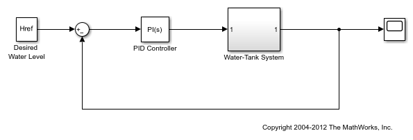
This example shows how to obtain multiple operating points for a model by varying parameter values. You can study the controller robustness to plant variations by batch linearizing the model using the trimmed operating points.
Open the Simulink model.
sys = 'watertank';
open_system(sys)

Vary parameters A and b within 10% of their nominal values. Specify three values for A and four values for b, creating a 3-by-4 value grid for each parameter.
[A_grid,b_grid] = ndgrid(linspace(0.9*A,1.1*A,3),...
                         linspace(0.9*b,1.1*b,4));
Create a parameter structure array, specifying the name and grid points for each parameter.
params(1).Name = 'A';
params(1).Value = A_grid;
params(2).Name = 'b';
params(2).Value = b_grid;
Create a default operating point specification for the model, which specifies that both model states are unknown and must be at steady state in the trimmed operating point.
opspec = operspec(sys)
opspec =


 Operating point specification for the Model watertank.
 (Time-Varying Components Evaluated at time t=0)

States:
----------
     x         Known    SteadyState     Min         Max        dxMin       dxMax
___________ ___________ ___________ ___________ ___________ ___________ ___________

(1.) watertank/PID Controller/Integrator/Continuous/Integrator
     0         false       true        -Inf         Inf        -Inf         Inf
(2.) watertank/Water-Tank System/H
     1         false       true          0          Inf        -Inf         Inf

Inputs: None
----------

Outputs: None
----------
By default, findop displays an operating point search report in the Command Window for each trimming operation. To suppress the report display, create a trimming option set and turn off the operating point search report display.
opt = findopOptions('DisplayReport','off');
Trim the model using the specified operating point specification, parameter grid, and option set.
[op,opreport] = findop(sys,opspec,params,opt);
findop trims the model for each parameter combination. The software uses only one model compilation. op is a 3-by-4 array of operating point objects that correspond to the specified parameter grid points.
View the operating point in the first row and first column of op.
op(1,1)
ans =


 Operating point for the Model watertank.
 (Time-Varying Components Evaluated at time t=0)

States:
----------
  x
______

(1.) watertank/PID Controller/Integrator/Continuous/Integrator
1.4055
(2.) watertank/Water-Tank System/H
  10

Inputs: None
----------
Batch Trim Model at Known States Derived from Parameter Values
This example shows how to batch trim a model when the specified parameter variations affect the known states for trimming.
In the Batch Trim Model for Parameter Variations example, the model is trimmed to meet a single operating point specification that contains unknown states. In other cases, the model states are known for trimming, but depend on the values of the varying parameters. In this case, you cannot batch trim the model using a single operating point specification. You must create a separate specification for each parameter value grid point.
Open the Simulink model.
sys = 'scdairframeTRIM';
open_system(sys)

In this model, the aerodynamic forces and moments depend on the speed,  , and incidence,
  .
.
Vary the  and
and  parameters, and create a 6-by-4 parameter grid.
nA = 6;    % number of alpha values
nV = 4;    % number of V values
alphaRange = linspace(-20,20,nA)*pi/180;
vRange = linspace(700,1400,nV);
[alphaGrid,vGrid] = ndgrid(alphaRange,vRange);
Since some known state values for trimming depend on the values of  and
and  , you must create a separate operating point specification object for each parameter combination.
for i = 1:nA
    for j = 1:nV
        % Set parameter values in model.
        alpha_ini = alphaGrid(i,j);
        v_ini = vGrid(i,j);

        % Create default specifications based on the specified parameters.
        opspec(i,j) = operspec(sys);

        % Specify which states are known and which states are at steady state.
        opspec(i,j).States(1).Known = [1;1];
        opspec(i,j).States(1).SteadyState = [0;0];

        opspec(i,j).States(3).Known = [1;1];
        opspec(i,j).States(3).SteadyState = [0;1];

        opspec(i,j).States(2).Known = 1;
        opspec(i,j).States(2).SteadyState = 0;

        opspec(i,j).States(4).Known = 0;
        opspec(i,j).States(4).SteadyState = 1;
    end
end
Create a parameter structure for batch trimming. Specify a name and value grid for each parameter.
params(1).Name = 'alpha_ini';
params(1).Value = alphaGrid;
params(2).Name = 'v_ini';
params(2).Value = vGrid;
Trim the model using the specified parameter grid and operating point specifications. When you specify an array of operating point specifications and varying parameter values, the dimensions of the specification array must match the parameter grid dimensions.
opt = findopOptions('DisplayReport','off');
op = findop(sys,opspec,params,opt);
findop trims the model for each parameter combination. op is a 6-by-4 array of operating point objects that correspond to the specified parameter grid points.
See Also
Topics
- Batch Compute Steady-State Operating Points for Multiple Specifications
- Batch Compute Steady-State Operating Points Reusing Generated MATLAB Code
- Batch Linearize Model at Multiple Operating Points Using linearize Command
- Vary Operating Points and Obtain Multiple Transfer Functions Using slLinearizer Interface