First-Cut Robust Design

Introduction

The plant model consists of a first-order system with uncertain gain and time constant in series with a mildly underdamped resonance and significant unmodeled dynamics. The uncertain variables are specified using ureal and ultidyn and the uncertain plant model P is constructed as a product of simple transfer functions:

gamma = ureal('gamma',2,'Perc',30);  % uncertain gain
tau = ureal('tau',1,'Perc',30);      % uncertain time-constant
wn = 50; xi = 0.25;
P = tf(gamma,[tau 1]) * tf(wn^2,[1 2*xi*wn wn^2]);
% Add unmodeled dynamics
delta = ultidyn('delta',[1 1],'SampleStateDim',5,'Bound',1);
W = makeweight(0.1,20,10);
P = P * (1+W*delta);

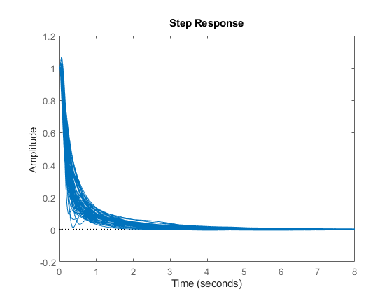
A collection of step responses for randomly sampled uncertainty values illustrates the plant variability.

step(P,5)

Covering the Uncertain Model

The uncertain plant model P contains 3 uncertain elements. For feedback design purposes, it is often desirable to simplify the uncertainty model while approximately retaining its overall variability. This is one use of the command ucover. This command takes an array of LTI responses Pa and a nominal response Pn and models the difference Pa-Pn as multiplicative uncertainty in the system dynamics (ultidyn).

To use ucover, first map the uncertain model P into a family of LTI responses using usample. This command samples the uncertain elements in an uncertain system. It returns an array of LTI models where each model representing one possible behavior of the uncertain system. In this example, generate 60 sample values of P:

rng('default');     % the random number generator is seeded for repeatability
Parray = usample(P,60);

Next, use ucover to cover all behaviors in Parray by a simple uncertain model of the form

Usys = Pn * (1 + Wt * Delta)

where all the uncertainty is concentrated in the "unmodeled dynamics" component Delta (a ultidyn object). Choose the nominal value of P as center Pn of the cover, and use a 2nd-order shaping filter Wt to capture how the relative gap between Parray and Pn varies with frequency.

Pn = P.NominalValue;
orderWt = 2;
Parrayg = frd(Parray,logspace(-3,3,60));
[Usys,Info] = ucover(Parrayg,Pn,orderWt,'in');

Verify that the filter magnitude (in red) "covers" the relative variations of the plant frequency response (in blue).

Wt = Info.W1;
bodemag((Pn-Parray)/Pn,'b--',Wt,'r')

Creating the Open-Loop Design Model

To design a robust controller for the uncertain plant P, choose a target closed-loop bandwidth desBW and perform a sensitivity-minimization design using the simplified uncertainty model Usys. The control structure is shown in Figure 1. The main signals are the disturbance d, the measurement noise n, the control signal u, and the plant output y. The filters Wperf and Wnoise reflect the frequency content of the disturbance and noise signals, or equivalently, the frequency bands where good disturbance and noise rejection properties are needed.

Our goal is to keep y close to zero by rejecting the disturbance d and minimizing the impact of the measurement noise n. Equivalently, we want to design a controller that keeps the gain from [d;n] to y "small." Note that

y  = Wperf * 1/(1+PC) * d + Wnoise * PC/(1+PC) * n

so the transfer function of interest consists of performance- and noise-weighted versions of the sensitivity function 1/(1+PC) and complementary sensitivity function PC/(1+PC).

Figure 1: Control Structure.

Choose the performance weighting function Wperf as a first-order low-pass filter with magnitude greater than 1 at frequencies below the desired closed-loop bandwidth:

desBW = 0.4;
Wperf = makeweight(500,desBW,0.5);

To limit the controller bandwidth and induce roll off beyond the desired bandwidth, use a sensor noise model Wnoise with magnitude greater than 1 at frequencies greater than 10*desBW:

Wnoise = 0.0025 * tf([25 7 1],[2.5e-5 .007 1]);

Plot the magnitude profiles of Wperf and Wnoise:

bodemag(Wperf,'b',Wnoise,'r'), grid
title('Performance weight and sensor noise model')
legend('Wperf','Wnoise','Location','SouthEast')

Next build the open-loop interconnection of Figure 1:

Usys.InputName = 'u'; Usys.OutputName = 'yp';
Wperf.InputName = 'd'; Wperf.OutputName = 'yd';
Wnoise.InputName = 'n'; Wnoise.OutputName = 'yn';

sumy = sumblk('y = yp + yd');
sume = sumblk('e = -y - yn');

M = connect(Usys,Wperf,Wnoise,sumy,sume,{'d','n','u'},{'y','e'});

First Design: Low Bandwidth Requirement

The controller design is carried out with the automated robust design command musyn. The uncertain open-loop model is given by M.

[ny,nu] = size(Usys);
[K1,muBound] = musyn(M,ny,nu);

D-K ITERATION SUMMARY:
-----------------------------------------------------------------
                       Robust performance               Fit order
-----------------------------------------------------------------
  Iter         K Step       Peak MU       D Fit             D
    1           223.6        100.5        101.4             2
    2            20.3        1.829        1.845            10
    3           1.009        1.001        1.012            10
    4          0.9545       0.9545       0.9627             8
    5          0.9349       0.9348       0.9379            10
    6          0.9249       0.9249       0.9268            10
    7          0.9207       0.9207       0.9235            10
    8           0.919        0.919       0.9193            10

Best achieved robust performance: 0.919

The robust performance muBound is a positive scalar. If it is near 1, then the design is successful and the desired and effective closed-loop bandwidths match closely. As a rule of thumb, if muBound is less than 0.85, then the achievable performance can be improved. When muBound is greater than 1.2, then the desired closed-loop bandwidth is not achievable for the given amount of plant uncertainty.

Since, here, muBound is approximately 0.9, the objectives are met, but could ultimately be improved upon. For validation purposes, create Bode plots of the open-loop response for different values of the uncertainty and note the typical zero-dB crossover frequency and phase margin:

opt = bodeoptions;
opt.PhaseMatching = 'on';
opt.Grid = 'on';

bodeplot(Parray*K1,{1e-2,1e2},opt);

Randomized closed-loop Bode plots confirm a closed-loop disturbance rejection bandwidth of approximately 0.4 rad/s.

S1 = feedback(1,Parray*K1);  % sensitivity to output disturbance
bodemag(S1,{1e-2,1e3}), grid

Finally, compute and plot the closed-loop responses to a step disturbance at the plant output. These are consistent with the desired closed-loop bandwidth of 0.4, with settling times approximately 7 seconds.

step(S1,8);

In this naive design strategy, we have correlated the noise bandwidth with the desired closed-loop bandwidth. This simply helps limit the controller bandwidth. A fair perspective is that this approach focuses on output disturbance attenuation in the face of plant model uncertainty. Sensor noise is not truly addressed. Problems with considerable amounts of sensor noise would be dealt with in a different manner.

Second Design: Higher Bandwidth Requirement

Let's redo the design for a higher target bandwidth and adjusting the noise bandwidth as well.

desBW = 2;
Wperf = makeweight(500,desBW,0.5);
Wperf.InputName = 'd'; Wperf.OutputName = 'yd';
Wnoise = 0.0025 * tf([1 1.4 1],[1e-6 0.0014 1]);
Wnoise.InputName = 'n'; Wnoise.OutputName = 'yn';

M = connect(Usys,Wperf,Wnoise,sumy,sume,{'d','n','u'},{'y','e'});
[K2,muBound2] = musyn(M,ny,nu);

D-K ITERATION SUMMARY:
-----------------------------------------------------------------
                       Robust performance               Fit order
-----------------------------------------------------------------
  Iter         K Step       Peak MU       D Fit             D
    1           223.6        100.5        101.5             2
    2           20.32        2.171        2.192            10
    3           1.275        1.268         1.28            10
    4            1.19         1.19        1.206            10
    5           1.165        1.165        1.171            10
    6           1.152        1.152        1.155            10
    7           1.142        1.142        1.145            10
    8           1.133        1.133        1.134            10
    9           1.127        1.127        1.128            10
   10           1.121        1.121        1.123            10

Best achieved robust performance: 1.12

With a robust performance of about 1.1, this design achieves a good tradeoff between performance goals and plant uncertainty. Open-loop Bode plots confirm a fairly robust design with decent phase margins, but not as good as the lower bandwidth design.

bodeplot(Parray*K2,{1e-2,1e2},opt)

Randomized closed-loop Bode plots confirm a closed-loop bandwidth of approximately 2 rad/s. The frequency response has a bit more peaking than was seen in the lower bandwidth design, due to the increased uncertainty in the model at this frequency. Since the Robust Performance mu-value was 1.1, we expected some degradation in the robustness of the performance objectives over the lower bandwidth design.

S2 = feedback(1,Parray*K2);
bodemag(S2,{1e-2,1e3}), grid

Closed-loop step disturbance responses further illustrate the higher bandwidth response, with reasonable robustness across the plant model variability.

step(S2,8);

Third Design: Very Aggressive Bandwidth Requirement

Redo the design once more with an extremely optimistic closed-loop bandwidth goal of 15 rad/s.

desBW = 15;
Wperf = makeweight(500,desBW,0.5);
Wperf.InputName = 'd'; Wperf.OutputName = 'yd';
Wnoise = 0.0025 * tf([0.018 0.19 1],[0.018e-6 0.19e-3 1]);
Wnoise.InputName = 'n'; Wnoise.OutputName = 'yn';

M = connect(Usys,Wperf,Wnoise,sumy,sume,{'d','n','u'},{'y','e'});
[K3,muBound3] = musyn(M,ny,nu);

D-K ITERATION SUMMARY:
-----------------------------------------------------------------
                       Robust performance               Fit order
-----------------------------------------------------------------
  Iter         K Step       Peak MU       D Fit             D
    1           223.6        100.9        101.9             2
    2           20.36        3.537        3.567             8
    3           2.152        2.152        2.177            10
    4           1.959        1.959        1.975            10
    5           1.884        1.884          1.9            10
    6           1.831        1.831        1.901             6
    7           1.811        1.811        1.833            10
    8           1.789        1.789        1.798             8
    9           1.771        1.771        1.783             8
   10           1.763        1.763        1.768             8

Best achieved robust performance: 1.76

Since the robust performance is greater than 1.8, the closed-loop performance goals are not achieved under plant uncertainties. The frequency responses of the closed-loop system have higher peaks indicating the poor performance of the designed controller.

S3 = feedback(1,Parray*K3);
bodemag(S3,{1e-2,1e3}), grid

Similarly, step responses under uncertainties illustrate the poor closed-loop performance.

step(S3,1);

Robust Stability Calculations

The Bode and Step response plots shown above are generated from samples of the uncertain plant model P. We can use the uncertain model directly, and assess the robust stability of the three closed-loop systems.

ropt = robOptions('Display','on','MussvOptions','sm5');
stabmarg1 = robstab(feedback(P,K1),ropt);

Computing peak...  Percent completed: 100/100
System is robustly stable for the modeled uncertainty.
 -- It can tolerate up to 271% of the modeled uncertainty.
 -- There is a destabilizing perturbation amounting to 272% of the modeled uncertainty.
 -- This perturbation causes an instability at the frequency 7.69 rad/seconds.

stabmarg2 = robstab(feedback(P,K2),ropt);

Computing peak...  Percent completed: 100/100
System is robustly stable for the modeled uncertainty.
 -- It can tolerate up to 148% of the modeled uncertainty.
 -- There is a destabilizing perturbation amounting to 148% of the modeled uncertainty.
 -- This perturbation causes an instability at the frequency 16.9 rad/seconds.

stabmarg3 = robstab(feedback(P,K3),ropt);

Computing peak...  Percent completed: 100/100
System is not robustly stable for the modeled uncertainty.
 -- It can tolerate up to 81.2% of the modeled uncertainty.
 -- There is a destabilizing perturbation amounting to 81.4% of the modeled uncertainty.
 -- This perturbation causes an instability at the frequency 82.7 rad/seconds.

The robustness analysis reports confirm what we have observed by sampling the closed-loop time and frequency responses. The second design is a good compromise between performance and robustness, and the third design is too aggressive and lacks robustness.