createPDEResults

R2026b

Create solution object

Syntax

results = createPDEResults(fem,u)

results = createPDEResults(fem,u,Name=Value)

pderesults = createPDEResults(pdem,pdeu)

pderesults = createPDEResults(pdem,pdeu,"stationary")

pderesults = createPDEResults(pdem,u,utimes,"time-dependent")

pderesults = createPDEResults(pdem,eigenvectors,eigenvalues,"eigen")

Description

results = createPDEResults(fem,u) creates a solution object from fem and its solution u.

results = createPDEResults(fem,u,Name=Value) creates a solution object using the Name=Value arguments.

pderesults = createPDEResults(pdem,pdeu) creates a StationaryResults solution object from pdem and its solution pdeu.

This syntax is equivalent to pderesults = createPDEResults(pdem,pdeu,"stationary").

Dimensions of the returned solutions and gradients are the same as those returned by solvepde. For details, see Dimensions of Solutions, Gradients, and Fluxes.

pderesults = createPDEResults(pdem,u,utimes,"time-dependent") creates a TimeDependentResults solution object from pdem, its solution pdeu, and the times utimes.

Dimensions of the returned solutions and gradients are the same as those returned by solvepde. For details, see Dimensions of Solutions, Gradients, and Fluxes.

pderesults = createPDEResults(pdem,eigenvectors,eigenvalues,"eigen") creates an EigenResults solution object from pdem, its eigenvector solution eigenvectors, and its eigenvalues eigenvalues

Dimensions of the returned solutions and gradients are the same as those returned by solvepdeeig. For details, see Dimensions of Solutions, Gradients, and Fluxes.

.

Examples

Create ElectrostaticResults Object

Create an ElectrostaticResults object to store the solution of an electrostatic analysis model.

Create a model for solving an electrostatic problem and assign the geometry of a cube to the model.

fem = femodel(AnalysisType="electrostatic", ...
    Geometry=multicuboid(0.1,0.1,0.1));

Generate a mesh.

fem = generateMesh(fem);

Specify relative permittivity of the material and vacuum permittivity.

fem.MaterialProperties = materialProperties( ...
    RelativePermittivity=2.5);
fem.VacuumPermittivity = 8.854e-12;

Create a custom solution representing the electric potential.

numNodes = size(fem.Mesh.Nodes,2);
u = rand(numNodes,1)*100;

Create the results object using the model and the custom solution.

results = createPDEResults(fem,u)

results = 
  ElectrostaticResults with properties:

      ElectricPotential: [34168×1 double]
          ElectricField: [1×1 FEStruct]
    ElectricFluxDensity: [1×1 FEStruct]
                   Mesh: [1×1 FEMesh]

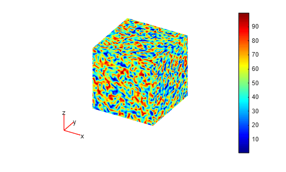
Plot the results.

pdeplot3D(fem.Mesh,ColorMapData=results.ElectricPotential)

Create TransientStructuralResults Object Specifying Displacement, Velocity, Acceleration, and Solution Times

Create a TransientStructuralResults object to store the solution of a transient structural analysis model.

Create a model for solving a transient structural analysis problem and assign the geometry of an L-shaped membrane to the model. Specify that the

model = femodel(AnalysisType="structuralTransient", ...
    Geometry=@lshapeg);

Specify the plane-stress problem type.

model.PlanarType = "planeStress";

Generate a mesh.

model = generateMesh(model);

Specify the Young's modulus, Poisson's ratio, and mass density of the material.

model.MaterialProperties = materialProperties(...
    YoungsModulus=210E9, ...
    PoissonsRatio=0.3, ...
    MassDensity=7850);

Create a vector of solution times.

numSteps = 4;
tlist = linspace(0,0.5,numSteps);

Create matrices representing a custom displacement, velocity, and acceleration.

numNodes = size(model.Mesh.Nodes,2);
u = rand(numNodes*2,numSteps);
dudt = rand(size(u));
dudt2 = rand(size(u));

Create the results object using the model and the custom solution.

results = createPDEResults(model,u, ...
Time=tlist, ...
Velocity=dudt, ...
Acceleration=dudt2)

results = 
  TransientStructuralResults with properties:

     Displacement: [1×1 FEStruct]
         Velocity: [1×1 FEStruct]
     Acceleration: [1×1 FEStruct]
    SolutionTimes: [0 0.1667 0.3333 0.5000]
             Mesh: [1×1 FEMesh]

Plot the y-component of the acceleration.

pdeplot(model.Mesh,XYData=results.Acceleration.ay)
axis equal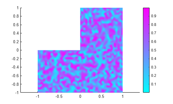

Results from an Elliptic Problem

Create a StationaryResults object from the solution to an elliptic system.

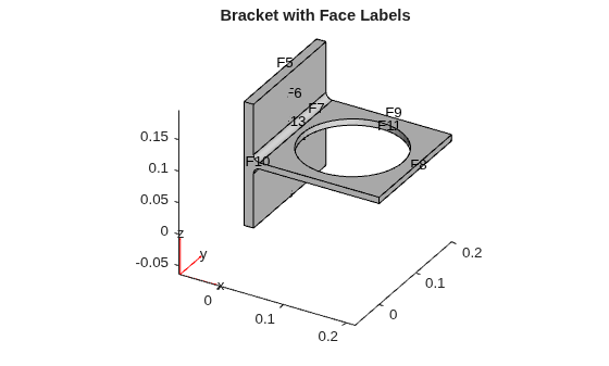
Create a PDE model for a system of three equations. Import the geometry of a bracket and plot the face labels.

model = createpde(3);
importGeometry(model,"BracketWithHole.stl");
figure
pdegplot(model,FaceLabels="on")
view(30,30)
title("Bracket with Face Labels")

figure
pdegplot(model,FaceLabels="on")
view(-134,-32)
title("Bracket with Face Labels, Rear View")

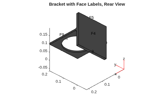
Set boundary conditions: face 3 is immobile, and there is a force in the negative z direction on face 6.

applyBoundaryCondition(model,"dirichlet",Face=4,u=[0,0,0]);
applyBoundaryCondition(model,"neumann",Face=8,g=[0,0,-1e4]);

Set coefficients that represent the equations of linear elasticity.

E = 200e9;
nu = 0.3;
c = elasticityC3D(E,nu);
a = 0;
f = [0;0;0];

Create a mesh and solve the problem.

generateMesh(model,Hmax=1e-2);
u = assempde(model,c,a,f);

Create a StationaryResults object from the solution.

results = createPDEResults(model,u)

results = 
  StationaryResults with properties:

    NodalSolution: [14093×3 double]
       XGradients: [14093×3 double]
       YGradients: [14093×3 double]
       ZGradients: [14093×3 double]
             Mesh: [1×1 FEMesh]

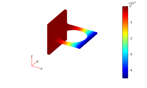
Plot the solution for the z-component, which is component 3.

pdeplot3D(model,ColorMapData=results.NodalSolution(:,3))

Results from a Time-Dependent Problem

Obtain a solution from a parabolic problem.

The problem models heat flow in a solid.

model = createpde();
importGeometry(model,"Tetrahedron.stl");
pdegplot(model,FaceLabels="on",FaceAlpha=0.5)
view(45,45)

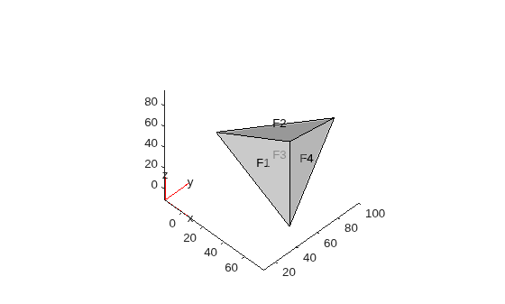
Set the temperature on face 2 to 100. Leave the other boundary conditions at their default values (insulating).

applyBoundaryCondition(model,"dirichlet",Face=2,u=100);

Set the coefficients to model a parabolic problem with 0 initial temperature.

d = 1;
c = 1;
a = 0;
f = 0;
u0 = 0;

Create a mesh and solve the PDE for times from 0 through 200 in steps of 10.

tlist = 0:10:200;
generateMesh(model);
u = parabolic(u0,tlist,model,c,a,f,d);

171 successful steps
0 failed attempts
329 function evaluations
1 partial derivatives
29 LU decompositions
328 solutions of linear systems

Create a TimeDependentResults object from the solution.

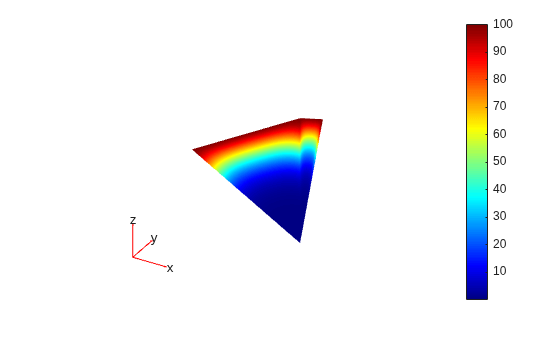
results = createPDEResults(model,u,tlist,"time-dependent");

Plot the solution on the surface of the geometry at time 100.

pdeplot3D(model,ColorMapData=results.NodalSolution(:,11))

Results from an Eigenvalue Problem

Create an EigenResults object from the solution to an eigenvalue problem.

Create the geometry and mesh for the L-shaped membrane. Apply Dirichlet boundary conditions to all edges.

model = createpde;
geometryFromEdges(model,@lshapeg);
generateMesh(model,Hmax=0.05,GeometricOrder="linear");
applyBoundaryCondition(model,"dirichlet", ...
                             Edge=1:model.Geometry.NumEdges, ...
                             u=0);

Solve the eigenvalue problem for coefficients c = 1, a = 0, and d = 1. Obtain solutions for eigenvalues from 0 through 100.

c = 1;
a = 0;
d = 1;
r = [0,100];
[eigenvectors,eigenvalues] = pdeeig(model,c,a,d,r);

Create an EigenResults object from the solution.

results = createPDEResults(model,eigenvectors,eigenvalues,"eigen")

results = 
  EigenResults with properties:

    Eigenvectors: [1458×12 double]
     Eigenvalues: [12×1 double]
            Mesh: [1×1 FEMesh]

Plot the solution for mode 10.

pdeplot(model,XYData=results.Eigenvectors(:,10))
axis equal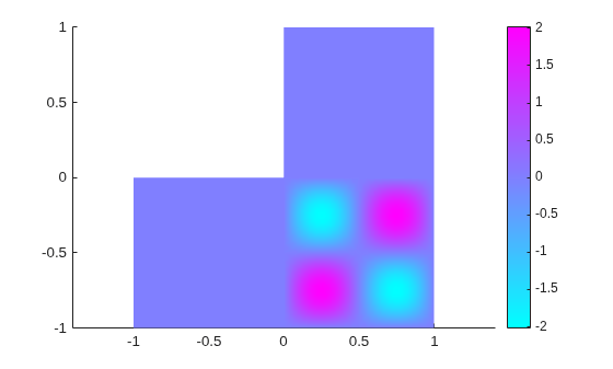

Input Arguments

fem — Finite element analysis model

femodel object

Finite element analysis model, specified as an femodel object. The model must contain the following information about a finite element problem: analysis type, geometry, material properties, and mesh. Depending on the analysis type, it represents a structural, thermal, or electromagnetic problem.

Example: fem = femodel(AnalysisType = "structuralStatic")

u — Solution to be stored in the results object

array

Solution to be stored in the results object, specified as an array. The size of the array depends on the analysis type and the mesh of the model. Specifically, the number of rows in u must be equal to the number of nodes in the mesh times the number of degrees of freedom per node. The number of columns in u varies accordingly to the analysis type: one column for steady-state analyses and one or more columns for all other types.

pdem — PDE model

PDEModel object

PDE model, specified as a PDEModel object.

Example: model = createpde

pdeu — PDE solution

vector | matrix

PDE solution, specified as a vector or matrix.

Example: pdeu = assempde(model,c,a,f);

utimes — Times for a PDE solution

monotone vector

Times for a PDE solution, specified as a monotone vector. These times should be the same as the tlist times that you specified for the solution by the hyperbolic or parabolic solvers.

Example: utimes = 0:0.2:5;

eigenvectors — Eigenvector solution

matrix

Eigenvector solution, specified as a matrix. Suppose

• Np is the number of mesh nodes

• N is the number of equations

• ev is the number of eigenvalues specified in eigenvalues

Then eigenvectors has size Np-by-N-by-ev. Each column of eigenvectors corresponds to the eigenvectors of one eigenvalue. In each column, the first Np elements correspond to the eigenvector of equation 1 evaluated at the mesh nodes, the next Np elements correspond to equation 2, and so on.

eigenvalues — Eigenvalue solution

vector

Eigenvalue solution, specified as a vector.

Name-Value Arguments

Specify optional pairs of arguments as Name1=Value1,...,NameN=ValueN, where Name is the argument name and Value is the corresponding value. Name-value arguments must appear after other arguments, but the order of the pairs does not matter.

Example: Frequency=linspace(0,4000,150)

Time — Solution times for structural or thermal transient analysis

real vector

Solution times for structural or thermal transient analysis, specified as a real vector of monotonically increasing or decreasing values.

Example: Time=0:20

Data Types: double

Frequency — Solution frequencies for frequency response structural analysis

real vector

Solution frequencies for a frequency response structural analysis, specified as a real vector of monotonically increasing or decreasing values.

Example: Frequency=linspace(0,4000,150)

Data Types: double

Eigenvalues — Eigenvalues for modal structural and thermal analysis

real vector

Eigenvalues for modal structural and thermal analysis, specified as a real vector. For structural analysis, the eigenvalues represent natural frequencies. For thermal analysis, they represent decay rates.

Example: Eigenvalues=[798;4989;13928;27177;44678]

Data Types: double

Velocity — Velocity vales at nodes

array

Velocity values at the nodes, specified as an array of the same size as the solution u.

Example: Velocity=rand(size(u))

Data Types: double

Acceleration — Acceleration vales at nodes

array

Acceleration values at the nodes, specified as an array of the same size as the solution u.

Example: Acceleration=rand(size(u))

Data Types: double

ModeType — Type of modes for modal thermal analysis

"EigenModes" (default) | "PODModes"

Type of modes for modal thermal analysis, specified as "EigenModes" or "PODModes".

Example: ModeType="PODModes"

Data Types: string

SnapshotsAverage — Average of snapshots for proper orthogonal decomposition (POD)

real array

Average of snapshots for POD, specified as a real array.

Data Types: double

Output Arguments

results — Structural, thermal, or electromagnetic analysis results

StaticStructuralResults object | TransientStructuralResults object | ModalStructuralResults object | FrequencyStructuralResults object | SteadyStateThermalResults object | TransientThermalResults object | ModalThermalResults object | ElectrostaticResults object | MagnetostaticResults object | ConductionResults object | HarmonicResults object

Structural, thermal, or electromagnetic analysis results. The type of the returned results object depends on the analysis type of the specified model, fem:

• If AnalysisType="structuralStatic", the returned object is StaticStructuralResults.

• If AnalysisType="structuralTransient", the returned object is TransientStructuralResults.

• If AnalysisType="structuralModal", the returned object is ModalStructuralResults.

• If AnalysisType="structuralFrequency", the returned object is FrequencyStructuralResults.

• If AnalysisType="thermalSteady", the returned object is SteadyStateThermalResults.

• If AnalysisType="thermalTransient", the returned object is TransientThermalResults.

• If AnalysisType="thermalModal", the returned object is ModalThermalResults.

• If AnalysisType="electrostatic", the returned object is ElectrostaticResults.

• If AnalysisType="magnetostatic", the returned object is MagnetostaticResults.

• If AnalysisType="dcConduction", the returned object is ConductionResults.

• If AnalysisType="electricHarmonic" or AnalysisType="magneticHarmonic", the returned object is HarmonicResults.

pderesults — PDE solution

StationaryResults object (default) | TimeDependentResults object | EigenResults object

PDE solution, specified as a StationaryResults object, a TimeDependentResults object, or an EigenResults object. Create pderesults using solvepde, solvepdeeig, or createPDEResults.

Example: pderesults = solvepde(pdem)

Version History

Introduced in R2015b

R2016a: No longer creates an object of type PDEResults

createPDEResults no longer creates an object of type PDEResults. The syntax of createPDEResults has changed to accommodate creating the new result types for time-dependent and eigenvalue problems.

• To create the TimeDependentResults object for a time-dependent problem, use the syntax createPDEResults(pdem,u,utimes,"time-dependent"), where utimes is a vector of solution times.

• To create the EigenResults object for an eigenvalue problem, use the syntax createPDEResults(pdem,eigenvectors,eigenvalues,"eigen").

EigenResults has different property names than PDEResults. Update any eigenvalue scripts that use PDEResults property names.