assembleFEMatrices

Assemble finite element matrices

Syntax

FEM = assembleFEMatrices(model)

FEM = assembleFEMatrices(model,matrices)

FEM = assembleFEMatrices(model,bcmethod)

FEM = assembleFEMatrices(___,state)

Description

FEM = assembleFEMatrices(model) returns a structural array containing all finite element matrices for a PDE problem specified as a model.

FEM = assembleFEMatrices(model,matrices) returns a structural array containing only the specified finite element matrices.

FEM = assembleFEMatrices(model,bcmethod) assembles finite element matrices and imposes boundary conditions using the method specified by bcmethod.

FEM = assembleFEMatrices(___,state) assembles finite element matrices using the input time or solution specified in the state structure array. The function uses the time field of the structure for time-dependent models and the solution field u for nonlinear models. You can use this argument with any of the previous syntaxes.

Examples

Finite Element Matrices for 2-D Problem

Create a PDE model for the Poisson equation on an L-shaped membrane with zero Dirichlet boundary conditions.

model = createpde;
geometryFromEdges(model,@lshapeg);
specifyCoefficients(model,m=0,d=0,c=1,a=0,f=1);
applyBoundaryCondition(model,"dirichlet", ...
                       edge=1:model.Geometry.NumEdges, ...
                       u=0);

Generate a mesh and obtain the default finite element matrices for the problem and mesh.

generateMesh(model,Hmax=0.2);
FEM = assembleFEMatrices(model)

FEM = struct with fields:
    K: [401×401 double]
    A: [401×401 double]
    F: [401×1 double]
    Q: [401×401 double]
    G: [401×1 double]
    H: [80×401 double]
    R: [80×1 double]
    M: [401×401 double]

Specified Set of Finite Element Matrices

Make computations faster by specifying which finite element matrices to assemble.

Create an femodel object for steady-state thermal analysis and include the geometry of the built-in function squareg.

model = femodel(AnalysisType="thermalSteady", ...
                Geometry=@squareg);

Plot the geometry with the edge labels.

pdegplot(model,EdgeLabels="on")
xlim([-1.1 1.1])
ylim([-1.1 1.1])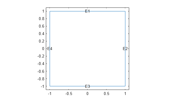

Specify the thermal conductivity of the material and the internal heat source.

model.MaterialProperties = ...
    materialProperties(ThermalConductivity=0.2);
model.FaceLoad = faceLoad(Heat=10);

Set the boundary conditions.

model.EdgeBC([1,3]) = edgeBC(Temperature=100);

Generate a mesh.

model = generateMesh(model);

Assemble the stiffness and mass matrices.

FEM_KM = assembleFEMatrices(model,"KM")

FEM_KM = struct with fields:
    K: [1529×1529 double]
    M: [1529×1529 double]

Now, assemble the finite element matrices M, K, A, and F.

FEM_MKAF = assembleFEMatrices(model,"MKAF")

FEM_MKAF = struct with fields:
    M: [1529×1529 double]
    K: [1529×1529 double]
    A: [1529×1529 double]
    F: [1529×1 double]

The four matrices M, K, A, and F correspond to discretized versions of the PDE coefficients m, c, a, and f. These four matrices also represent the domain of the finite-element model of the PDE. Instead of specifying them explicitly, you can use the domain argument.

FEMd = assembleFEMatrices(model,"domain")

FEMd = struct with fields:
    M: [1529×1529 double]
    K: [1529×1529 double]
    A: [1529×1529 double]
    F: [1529×1 double]

The four matrices Q, G, H, and R, correspond to discretized versions of q, g, h, and r in the Neumann and Dirichlet boundary condition specification. These four matrices also represent the boundary of the finite-element model of the PDE. Use the boundary argument to assemble only these matrices.

FEMb = assembleFEMatrices(model,"boundary")

FEMb = struct with fields:
    H: [74×1529 double]
    R: [74×1 double]
    G: [1529×1 double]
    Q: [1529×1529 double]

Finite Element Matrices with nullspace and stiff-spring Methods

Create a PDE model for the Poisson equation on an L-shaped membrane with zero Dirichlet boundary conditions.

model = createpde;
geometryFromEdges(model,@lshapeg);
specifyCoefficients(model,m=0,d=0,c=1,a=0,f=1);
applyBoundaryCondition(model,"dirichlet", ...
                       Edge=1:model.Geometry.NumEdges, ...
                       u=0);

Generate a mesh.

generateMesh(model,Hmax=0.2);

Obtain the finite element matrices after imposing the boundary condition using the null-space approach. This approach eliminates the Dirichlet degrees of freedom and provides a reduced system of equations.

FEMn = assembleFEMatrices(model,"nullspace")

FEMn = struct with fields:
    Kc: [321×321 double]
    Fc: [321×1 double]
     B: [401×321 double]
    ud: [401×1 double]
     M: [321×321 double]

Obtain the solution to the PDE using the nullspace finite element matrices.

un = FEMn.B*(FEMn.Kc\FEMn.Fc) + FEMn.ud;

Compare this result to the solution given by solvepde. The two solutions are identical.

u1 = solvepde(model);
norm(un - u1.NodalSolution)

ans = 
0

Obtain the finite element matrices after imposing the boundary condition using the stiff-spring approach. This approach retains the Dirichlet degrees of freedom, but imposes a large penalty on them.

FEMs = assembleFEMatrices(model,"stiff-spring")

FEMs = struct with fields:
    Ks: [401×401 double]
    Fs: [401×1 double]
     M: [401×401 double]

Obtain the solution to the PDE using the stiff-spring finite element matrices. This technique gives a less accurate solution.

us = FEMs.Ks\FEMs.Fs;
norm(us - u1.NodalSolution)

ans = 
0.0098

Finite Element Matrices for Time-Dependent Problem

Assemble finite element matrices for the first and last time steps of a transient structural problem.

Create the geometry and plot a cylinder geometry.

gm = multicylinder(0.01,0.05);
addVertex(gm,Coordinates=[0,0,0.05]);
pdegplot(gm,FaceLabels="on",FaceAlpha=0.5)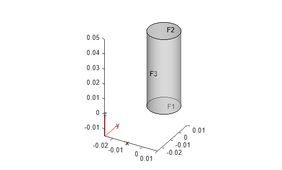

Create an femodel object for transient structural analysis and include the geometry in the model.

model = femodel(AnalysisType="structuralTransient", ...
                Geometry=gm);

Specify Young's modulus and Poisson's ratio.

model.MaterialProperties = ...
    materialProperties(YoungsModulus=201E9, ...
                       PoissonsRatio=0.3, ...
                       MassDensity=7800);

Specify that the bottom of the cylinder is a fixed boundary.

model.FaceBC(1) = faceBC(Constraint="fixed");

Create a function specifying a harmonic pressure load.

function Tn = sinusoidalLoad(load,location,state,Frequency,Phase)
if isnan(state.time)
    Tn = NaN*(location.nx);
    return
end
if isa(load,"function_handle")
    load = load(location,state);
else
    load = load(:);
end
% Transient model excited with harmonic load
Tn = load.*sin(Frequency.*state.time + Phase);
end

Apply the harmonic pressure on the top of the cylinder.

Pressure = 5e7;
Frequency = 50;
Phase = 0;
pressurePulse = @(location,state) ...
         sinusoidalLoad(Pressure,location,state,Frequency,Phase);
model.FaceLoad(2) = faceLoad(Pressure=pressurePulse);

Specify the zero initial displacement and velocity.

model.CellIC = cellIC(Displacement=[0;0;0], ...
                      Velocity=[0;0;0]);

Generate a linear mesh.

model = generateMesh(model,GeometricOrder="linear");

Assemble the finite element matrices for the initial time step.

tlist = linspace(0,1,300);
state.time = tlist(1);
FEM_domain = assembleFEMatrices(model,state)

FEM_domain = struct with fields:
    K: [6645×6645 double]
    A: [6645×6645 double]
    F: [6645×1 double]
    Q: [6645×6645 double]
    G: [6645×1 double]
    H: [252×6645 double]
    R: [252×1 double]
    M: [6645×6645 double]

Pressure applied at the top of the cylinder is the only time-dependent quantity in the model. To model the dynamics of the system, assemble the boundary-load finite element matrix G for the initial, intermediate, and final time steps.

state.time = tlist(1);
FEM_boundary_init = assembleFEMatrices(model,"G",state)

FEM_boundary_init = struct with fields:
    G: [6645×1 double]

state.time = tlist(floor(length(tlist)/2));
FEM_boundary_half = assembleFEMatrices(model,"G",state)

FEM_boundary_half = struct with fields:
    G: [6645×1 double]

state.time = tlist(end);
FEM_boundary_final = assembleFEMatrices(model,"G",state)

FEM_boundary_final = struct with fields:
    G: [6645×1 double]

Finite Element Matrices for Nonlinear Problem

Assemble finite element matrices for a heat transfer problem with temperature-dependent thermal conductivity.

Create a 2-D geometry by drawing one rectangle the size of the block and a second rectangle the size of the slot.

r1 = [3 4 -.5 .5 .5 -.5  -.8 -.8 .8 .8];
r2 = [3 4 -.05 .05 .05 -.05  -.4 -.4 .4 .4];
gdm = [r1; r2]';

Subtract the second rectangle from the first to create the block with a slot.

g = decsg(gdm,'R1-R2',['R1'; 'R2']');

Create an femodel object for steady-state thermal analysis and include the geometry in the model.

model = femodel(AnalysisType="thermalSteady", ...
                        Geometry=g);

Plot the geometry.

pdegplot(model,EdgeLabels="on"); 
axis([-.9 .9 -.9 .9]);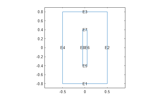

Set the temperature on the left edge to 100 degrees. Set the heat flux out of the block on the right edge to -10. The top and bottom edges and the edges inside the cavity are all insulated: there is no heat transfer across these edges.

model.EdgeBC(6) = edgeBC(Temperature=100);
model.EdgeLoad(1) = edgeLoad(Heat=-10);

Specify the thermal conductivity of the material as a simple linear function of temperature u.

k = @(~,state) 0.7+0.003*state.u;
model.MaterialProperties = ...
    materialProperties(ThermalConductivity=k);

Specify the initial temperature.

model.FaceIC = faceIC(Temperature=0);

Generate a mesh.

model = generateMesh(model);

Calculate the steady-state solution.

Rnonlin = solve(model);

Because the thermal conductivity is nonlinear (depends on the temperature), compute the system matrices corresponding to the converged temperature. Assign the temperature distribution to the u field of the state structure array. Because the u field must contain a row vector, transpose the temperature distribution.

state.u = Rnonlin.Temperature.';

Assemble finite element matrices using the temperature distribution at the nodal points.

FEM = assembleFEMatrices(model,"nullspace",state)

FEM = struct with fields:
    Kc: [1285×1285 double]
    Fc: [1285×1 double]
     B: [1308×1285 double]
    ud: [1308×1 double]
     M: [1285×1285 double]

Compute the solution using the system matrices to verify that they yield the same temperature as Rnonlin.

u = FEM.B*(FEM.Kc\FEM.Fc) + FEM.ud; 

Compare this result to the solution given by solve.

norm(u - Rnonlin.Temperature)

ans = 
1.8555e-06

Input Arguments

model — Model object

femodel object | PDEModel object

Model object, specified as an femodel or PDEModel object.

assembleFEMatrices does not support assembling FE matrices for 3-D magnetostatic analysis.

Example: model = femodel

Example: model = createpde

bcmethod — Method for including boundary conditions

"none" (default) | "nullspace" | "stiff-spring"

Method for including boundary conditions, specified as "none", "nullspace", or "stiff-spring". For more information, see Algorithms.

Example: FEM = assembleFEMatrices(model,"nullspace")

Data Types: char | string

matrices — Matrices to assemble

matrix identifiers | "boundary" | "domain"

Matrices to assemble, specified as:

• Matrix identifiers, such as "F", "MKF", "K", and so on — Assemble the corresponding matrices. Each uppercase letter represents one matrix: K, A, F, Q, G, H, R, M, and T. You can combine several letters into one character vector or string, such as "MKF".

• "boundary" — Assemble all matrices related to geometry boundaries.

• "domain" — Assemble all domain-related matrices.

Example: FEM = assembleFEMatrices(model,"KAF")

Data Types: char | string

state — Time for time-dependent models and solution for nonlinear models

structure array

Time for time-dependent models and solution for nonlinear models, specified in a structure array. The array fields represent the following values:

• state.time contains a nonnegative number specifying the time value for time-dependent models.

• state.u contains a solution matrix of size N-by-Np that can be used to assemble matrices in a nonlinear problem setup, where coefficients are functions of state.u. Here, N is the number of equations in the system, and Np is the number of nodes in the mesh.

Example: state.time = tlist(end); FEM = assembleFEMatrices(model,"boundary",state)

Output Arguments

FEM — Finite element matrices

structural array

Finite element matrices, returned as a structural array. Use the bcmethod and matrices arguments to specify which finite element matrices you want to assemble.

The fields in the structural array depend on bcmethod:

• If the value is "none", then the fields are K, A, F, Q, G, H, R, and M.

• If the value is "nullspace", then the fields are Kc, Fc, B, ud, and M.

• If the value is "stiff-spring", then the fields are Ks, Fs, and M.

The fields in the structural array also depend on matrices:

• If the value is boundary, then the fields are all matrices related to geometry boundaries.

• If the value is domain, then the fields are all domain-related matrices.

• If the value is a matrix identifier or identifiers, such as "F", "MKF", "K", and so on, then the fields are the corresponding matrices.

For more information, see Algorithms.

Algorithms

Partial Differential Equation Toolbox™ solves equations of the form

$$m\frac{{\partial }^{2}u}{\partial t^2}+d\frac{\partial u}{\partial t}-\nabla ·\left(c\otimes \nabla u\right)+au=f$$

and eigenvalue equations of the form

$$\begin{array}{l}-\nabla ·\left(c\otimes \nabla u\right)+au=\lambda du\\ \text{or}\\ -\nabla ·\left(c\otimes \nabla u\right)+au={\lambda }^{2}mu\end{array}$$

with the Dirichlet boundary conditions, hu = r, and Neumann boundary conditions, $$n·\left(c\otimes \nabla u\right)+qu=g$$.

assembleFEMatrices returns the following full finite element matrices and vectors that represent the corresponding PDE problem:

• K is the stiffness matrix, the integral of the discretized version of the c coefficient.

• M is the mass matrix, the integral of the discretized version of the m or d coefficients. M is nonzero for time-dependent and eigenvalue problems.

• A is the integral of the discretized version of the a coefficient.

• F is the integral of the discretized version of the f coefficient. For thermal, electromagnetic, and structural problems, F is a source or body load vector.

• Q is the integral of the discretized version of the q term in a Neumann boundary condition.

• G is the integral of the discretized version of the g term in a Neumann boundary condition. For structural problems, G is a boundary load vector.

• The H and R matrices come directly from the Dirichlet conditions and the mesh.

Imposing Dirichlet Boundary Conditions

The "nullspace" technique eliminates Dirichlet conditions from the problem using a linear algebra approach. It generates the combined finite-element matrices Kc, Fc, B, and vector ud corresponding to the reduced system Kc*u = Fc, where Kc = B'*(K + A + Q)*B, and Fc = B'*((F + G)-(K + A + Q)*ud). The B matrix spans the null space of the columns of H (the Dirichlet condition matrix representing h*ud = r). The R vector represents the Dirichlet conditions in H*ud = R. The ud vector has the size of the solution vector. Its elements are zeros everywhere except at Dirichlet degrees-of-freedom (DoFs) locations where they contain the prescribed values.

From the "nullspace" matrices, you can compute the solution u as

u = B*(Kc\Fc) + ud.

If you assembled a particular set of matrices, for example G and M, you can impose the boundary conditions on G and M as follows. First, compute the nullspace of columns of H.

[B,Or] = pdenullorth(H);
ud = Or*((H*Or\R)); % Vector with known value of the constraint DoF.

Then use the B matrix as follows. To eliminate Dirichlet degrees of freedom from the load vector G, use:

GwithBC = B'*G

To eliminate Dirichlet degrees of freedom from mass matrix, use:

M = B'*M*B

You can eliminate Dirichlet degrees of freedom from other vectors and matrices using the same technique.

The "stiff-spring" technique converts Dirichlet boundary conditions to Neumann boundary conditions using a stiff-spring approximation. It returns a matrix Ks and a vector Fs that together represent a different type of combined finite element matrices. The approximate solution is u = Ks\Fs. Compared to the "nullspace" technique, the "stiff-spring" technique generates matrices more quickly, but generally gives less accurate solutions.

Note

Internally, the toolbox uses the "nullspace" approach to impose Dirichlet boundary conditions while computing the solution using solvepde and solve.

Degrees of Freedom (DoFs)

If the number of nodes in a model is NumNodes, and the number of equations is N, then the length of column vectors u and ud is N*NumNodes. The toolbox assigns the IDs to the degrees of freedom in u and ud:

• Entries from 1 to NumNodes correspond to the first equation.

• Entries from NumNodes+1 to 2*NumNodes correspond to the second equation.

• Entries from 2*NumNodes+1 to 3*NumNodes correspond to the third equation.

The same approach applies to all other entries, up to N*NumNodes.

For example, in a 3-D structural model, the length of a solution vector u is 3*NumNodes. The first NumNodes entries correspond to the x-displacement at each node, the next NumNodes entries correspond to the y-displacement, and the next NumNodes entries correspond to the z-displacement.

Thermal, Structural, and Electromagnetic Analysis

In thermal analysis, the m and a coefficients are zeros. The thermal conductivity maps to the c coefficient. The product of the mass density and the specific heat maps to the d coefficient. The internal heat source maps to the f coefficient. The temperature on a boundary corresponds to the Dirichlet boundary condition term r with h = 1. Various forms of boundary heat flux, such as the heat flux itself, emissivity, and convection coefficient, map to the Neumann boundary condition terms q and g.

In structural analysis, the a coefficient is zero. Young's modulus and Poisson's ratio map to the c coefficient. The mass density maps to the m coefficient. The body loads map to the f coefficient. Displacements, constraints, and components of displacement along the axes map to the Dirichlet boundary condition terms h and r. Boundary loads, such as pressure, surface tractions, and translational stiffnesses, correspond to the Neumann boundary condition terms q and g. When you specify the damping model by using the Rayleigh damping parameters Alpha and Beta, the discretized damping matrix C is computed by using the mass matrix M and the stiffness matrix K as C = Alpha*M + Beta*K. Hysteretic (structural) damping contributes to the stiffness matrix K, which becomes complex.

In electrostatic and magnetostatic analyses, the m, a, and d coefficients are zeros. The relative permittivity and relative permeability map to the c coefficient. The charge density and current density map to the f coefficient. The voltage and magnetic potential on a boundary correspond to the Dirichlet boundary condition term r with h = 1.

Note

Assembling FE matrices does not work for harmonic analysis and 3-D magnetostatic analysis.

Version History

Introduced in R2016a

R2025a: To be removed: structural, thermal, and electromagnetic analysis models

assembleFEMatrices will no longer accept StructuralModel, ThermalModel, and ElectromagneticModel. These objects will be removed. Use an femodel object instead.

The unified finite element model workflow defines the type of a problem and all of its parameters as the properties of an femodel object. This object enables you to specify physical parameters for structural, thermal, and electromagnetic types of analyses. The solver in the unified workflow uses only the parameters (properties) appropriate for the current analysis type while ignoring all other properties. If you switch the analysis type by setting the AnalysisType property of the model, the solver uses the appropriate set of properties corresponding to the new analysis type.

For more help migrating your existing code that uses StructuralModel, ThermalModel, or ElectromagneticModel to the unified finite element workflow, see Migration from Domain-Specific to Unified Workflow.

R2024a: FE matrices for femodel

The function accepts femodel objects used in Unified Modeling.

R2020b: FE matrices for time-dependent and nonlinear models

The function now can assemble matrices using input time or solution for a time-dependent or nonlinear model, respectively. It also can assemble a subset of matrices, such as updated load only or stiffness only, to save computation time.

R2019a: FE matrices for thermal and structural models

The function accepts thermal and structural models with time- and solution-independent coefficients.