Optimization Explorer

Explore multiple solver configurations and their solutions for an optimization problem

Since R2026a

Description

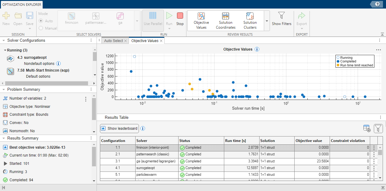
The Optimization Explorer app uses multiple solver configurations (solvers, options, and start points) to search for a global solution to an optimization problem. Using auto mode, you can repeatedly search for a global solution to an optimization problem, or search for the best combination of solver and options to solve an optimization problem. Using manual mode, you can create a set of solvers, initial conditions, and options to explore. By default, Optimization Explorer plots and stores the results. To explore further, you can run additional optimizations in the current session or a previous session.

Note

To use Optimization Explorer, you must first create an optimization problem. You can provide an OptimizationProblem object using MATLAB^® commands, or define an OptimizationProblem object using the problem-based Optimize Live Editor task. You can also provide the inputs to an optimization solver, such as fmincon or patternsearch, as variables in your workspace. Providing an OptimizationProblem object gives Optimization Explorer the most information about your problem, enabling the app to find the solution most efficiently.

Open the Optimization Explorer App

• MATLAB Toolstrip: On the Apps tab, under Math, Statistics and Optimization, click the app icon.

• MATLAB command prompt: Enter optimizationExplorer.

Examples

• Use Optimization Explorer App
• Optimize Simulink Model in Parallel with Optimization Explorer (Global Optimization Toolbox)

Parameters

Optimization Parameters

Problem Object — Optimization problem expressed in optimization variables

OptimizationProblem object

When you specify the problem as an OptimizationProblem object, Optimization Explorer has the most data and can, therefore, choose the most appropriate solvers.

Create a Problem Object using the Problem-Based Optimization Workflow. Begin by calling optimproblem, and then add the objective function and constraints.

Alternatively, create a Problem Object using the problem-based version of the Optimize Live Editor task.

Solver Inputs — Data for solver inputs

fmincon solver inputs | fminunc solver inputs | fminsearch solver inputs | lsqnonlin solver inputs | ga solver inputs | patternsearch solver inputs | particleswarm solver inputs | surrogateopt solver inputs

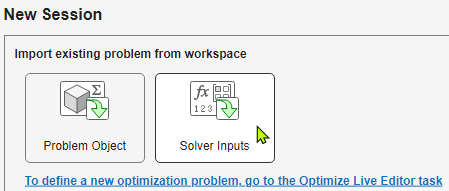
When you specify the problem using solver inputs, Optimization Explorer has less data than if you specify the problem using optimization variables, so the solution process can be less efficient. The solvers and their syntaxes are listed in these links:

• fmincon

• fminunc

• fminsearch

• lsqnonlin

• ga (Global Optimization Toolbox)

• patternsearch (Global Optimization Toolbox)

• particleswarm (Global Optimization Toolbox)

• surrogateopt (Global Optimization Toolbox)

Create solver inputs at the command line. Typical inputs include:

• Objective function — Create a function handle such as @fun. See Writing Scalar Objective Functions.

• Nonlinear constraint function — Create a function handle such as @nlcon. See Nonlinear Constraints.

• Initial point x0 — Create a row vector or other array. See x0.

• Lower bound lb and upper bound ub — Create a numeric vector or array. See Bound Constraints.

• Linear constraints — Create a numeric matrix A and corresponding vector b for inequality constraints, and create a numeric matrix Aeq and corresponding vector beq for equality constraints. See Linear Constraints.

x0 — Initial point

double array | structure | OptimizationValues object

Specify the initial point for the solver according to the following guidelines.

• New Session: x0 indicates the number and shape of the optimization variables.

  • Solver Inputs — Specify x0 as a real vector or array for solvers that requires an initial point, such as fmincon. The objective function fun must be able to evaluate fun(x0) and return a scalar value (or, for the lsqnonlin solver, a vector value).

  • Problem Object — x0 is not required because the problem object contains information about the number and shape of the variables.

• Manual Mode: Solvers use any specified start points.

  • Solver Inputs for single-point objective — Specify x0 as an array with the number of elements is equal to the number of problem variables.

  • Solver Inputs for multistart or population-based objective — Specify x0 as a matrix where each row represents one point and the number of columns is the number of problem variables. A population-based solver uses more than one point to evaluate the objective function, such as ga or particleswarm.

  • Problem Object for single-point objective — Specify x0 as a structure whose field names match the problem variable names. For example, if your problem has optimization variables "x" and "angle", the structure x0 must include the fields x0.x and x0.angle, specified as real arrays.

  • Problem Object for multistart or population-based objective — Specify x0 as a structure as for a single-point objective or as an OptimizationValues vector. Optimization Explorer uses only the Variables property of the OptimizationValues object, not any Objective or Constraints values.

Problem Attribute Parameters

Convex — Indication that the optimization problem is convex

Unsure (default) | Yes | No

Specify whether the optimization problem is convex.

Solvers use special techniques to optimize convex functions and, with convex constraints, any local minimum is a global minimum. Select Yes only if you are sure that your problem (including both the objective function and the constraints) is convex.

Nonsmooth — Indication that optimization problem is nonsmooth

Unsure (default) | Yes | No

Specify whether the optimization problem is nonsmooth.

A nonsmooth function has jumps or kinks, causing it to lack derivatives at some points. Some solvers require derivatives and, therefore, cannot handle a nonsmooth function. Select Yes only if you are sure that your objective function is nonsmooth or the nonlinear constraints are nonsmooth.

Simulation — Indication that objective function or nonlinear constraints come from a simulation

Unsure (default) | Yes | No

Specify whether the objective function or nonlinear constraints come from a simulation.

A simulation computes an objective or nonlinear constraint function by numerically solving a differential equation, or by using complex code such as Simulink^®. Simulations are typically expensive (time-consuming) and are often nonsmooth.

Note

Currently, parallel processing is not supported for problems that use a Simulink model. For a workaround, see Optimize Simulink Model in Parallel with Optimization Explorer (Global Optimization Toolbox).

Expensive — Indication that objective function or nonlinear constraints are time-consuming

Unsure (default) | Yes | No

Specify whether the objective function or nonlinear constraints are time-consuming to evaluate, or expensive.

An expensive function takes roughly five seconds or longer to evaluate. Some solvers are well suited to expensive functions. Select Yes when your objective function and nonlinear constraints combined typically take at least five seconds to evaluate at one point.

Select Solver Parameters

Mode — Optimization Explorer operational mode

Auto (default) | Manual

Specify the operational mode for the Optimization Explorer app.

• Auto mode causes the app to repeatedly run applicable solvers from a variety of start points or random seeds up to a stopping condition, such as a time limit you set. See Stopping Conditions.

• Manual mode causes the app to run the solver configurations you set manually. The available solvers depend on the problem type. For the list of potential solvers, see Solver.

Solver — Solver to use

fmincon | fminunc | fminsearch | lsqnonlin | patternsearch | ga | particleswarm | surrogateopt | multistart fmincon | multistart fminsearch | multistart fminunc | multistart lsqnonlin | multistart patternsearch

Specify one of the following as the solver to use:

• fmincon

• fminsearch

• fminunc

• lsqnonlin

• patternsearch (Global Optimization Toolbox)

• ga (Global Optimization Toolbox)

• particleswarm (Global Optimization Toolbox)

• simulannealbnd (Global Optimization Toolbox)

• surrogateopt (Global Optimization Toolbox)

• multistart fmincon

• multistart fminsearch

• multistart fminunc

• multistart lsqnonlin

• multistart patternsearch

The multistart solvers allow you to run multiple instances of the same solver and options using different start points.

Note

The multistart solvers do not run the MultiStart (Global Optimization Toolbox) solver. Instead, they run the named solver multiple times using randomly selected start points within the problem bounds. Optimization Explorer creates uniformly random start points, and uses artificial bounds of ±1000 for unbounded components.

Run Parameters

Use Parallel — Parallel processing type

false (default) | true

Specify whether to use parallel processing (true) or serial processing (false). To run in parallel, you must have Parallel Computing Toolbox™.

When processing in parallel, the app generally allocates one configuration per parallel worker, simultaneously processing several configurations at once. Parallel processing is usually faster than serial processing.

Note

Currently, parallel processing is not supported for problems that use a Simulink model. For a workaround, see Optimize Simulink Model in Parallel with Optimization Explorer (Global Optimization Toolbox).

Run — Start Optimization Explorer

Run (default) | Run next

Specify how to start Optimization Explorer. The effect of this parameter depends on the Mode setting.

• Auto mode — When you select Run or Run next, the app chooses the solver configurations to run until it reaches a stopping condition.

• Manual mode — When you select Run, the app runs the scheduled configurations. When you select Run next, the app runs only the next scheduled configuration. You can see the scheduled configurations in the Solver Configurations panel.

Review Results Parameters

Objective Values — Scatter plot of objective function values against solver run time

true (default)

Display a scatter plot (the default plot) of the objective function values against solver run time.

• The time axis is log-scaled. The objective function axis is unscaled (linear).

• To view details of a plotted point, click a point to activate data tips. Click the point again to hide the data tips.

• The display is affected by the filter and leaderboard settings.

Solution Coordinates — Parallel coordinates plot of solutions

false (default)

Display a parallel coordinates plot of solutions, similar to parallelplot. To see the results more easily when the plot has different coordinate scales, select Rescale values to have each coordinate value lie in the interval [0,1].

• Plotted points and lines are colored by the objective function value, as shown in the accompanying color bar.

• To view details of a plotted solution, click a point to activate data tips. Click the point again to hide the data tips.

• The display is affected by the filter and leaderboard settings.

Solution Clusters — Scatter plot or t-SNE plot of solution clusters

false (default)

Display a scatter plot or t-SNE plot of solution clusters, depending on the number of dimensions of the solution points. For solutions with one or two dimensions, the app displays a scatter plot. For solutions with three or more dimensions, the app displays a t-SNE plot of solution clusters, as returned by tsne (Statistics and Machine Learning Toolbox).

• Plotted markers are colored by the objective function value, as shown in the accompanying color bar.

• To view details of a plotted solution, click a point to activate data tips. Click the point again to hide the data tips.

• The display is affected by the filter and leaderboard settings.

Spider Plot — Spider plot of solutions

false (default)

Display a spider plot of solutions along five axes of these quantities for each solution:

• Objective value — Objective function value

• Run time [s] — Run time in seconds

• Constraint violation — Infeasibility (maximum constraint violation)

• Function evaluations — Number of function evaluations

• Optimality — First-Order Optimality Measure (applies only to Optimization Toolbox™ solvers)

Note the following:

• Plotted points and lines are colored by the objective function value, as shown in the accompanying color bar.

• To view details of a plotted solution, click a point to activate data tips. Click the point again to hide the data tips.

• The display is affected by the filter and leaderboard settings.

Solver Box Plot — Box plot of objective function values by solver algorithm

false (default)

Display a box plot of objective function values by solver algorithm, as returned by boxchart.

• To view details of a plotted solution, hover your cursor over the point of interest. Click the point to have the data tip remain. Hover or click on other points of interest to have them display simultaneously. Click a black anchor point to hide the data tip.

• The display is affected by the filter and leaderboard settings.

Show Filters — Toggle display of filter options

Off (default) | On

Toggle the display of the Results Filters panel. The options in this panel allow you to filter the results that appear in the plots and the Results Table, specifically the:

• Selected solvers

• Selected status (Completed, Run time limit reached, or Stopped)

• Results that fall within the specified range for Run time, Objective value, or Constraint violation

The Results Filters panel shows the number of currently visible results and the total number of results.

The Results Table shows the same information. To remove the filters, click the button.

Show Leaderboard — Show top results sorted by objective value

Off (default) | On

Show the top results sorted by objective value. The leaderboard contains up to 10 results. To cancel the leaderboard, click the button.

The leaderboard is not available when another filter is active.

Export Parameters

Export — Export results to workspace

Export Results Table (default) | Export Function

Specify how to export results to the workspace.

• Export Results Table exports a table of results as currently filtered.

• Export Function exports a function that reproduces the results of the selected row in the Results Table. To run this function, you generally need the original optimization problem as an input, or the solver inputs you originally used to create the session. If you used solver inputs, the exported function requires you to pass in all solver inputs, even those that were unused. Pass empty brackets ([]) for each unused input in the exported function.

Programmatic Use

optimizationExplorer opens the Optimization Explorer app or brings focus to the app if it is already open.

optimizationExplorer(folder) opens the Optimization Explorer app with the previously saved session in folder. The folder argument, specified as a character vector or string scalar, must include the name of an Optimization Explorer session folder and the path to the folder, if the session folder is not in the current folder.

Limitations

Supported Problem Types

Optimization Explorer currently solves only explicitly nonlinear problems that are not quadratic. Specifically, Optimization Explorer does not support:

• Linear programming problems

• Quadratic programming problems

• Cone programming problems

• Multiobjective problems

• Mixed-integer linear programming problems

Linear programming, convex quadratic programming, and cone programming problems have unique optimal objective function values, so Optimization Explorer is not the right tool for solving these problems. For linear programming problems, the linprog sensitivity output gives more information than Optimization Explorer about the effects of changing the problem parameters.

Session Folders are Not Protected

When you save an Optimization Explorer session using Save or Save as, the resulting folder is not protected from change. If any file in the session folder is changed, either in name or in its contents, then you might not be able to reopen the session. In other words, to be able to use a session folder to restart an Optimization Explorer session, do not change anything in the folder.

Tips

• As a best practice, run a solver on your problem once before running the solver in Optimization Explorer. This procedure ensures that a solver can run your problem without error.

• When you run additional solver configurations, the app retains the current results and adds the new results to the Results Table and plots.

• The options for displaying plots and filtering results are active during a run, as is the Stop button on the toolstrip. However, the effects of these options might seem delayed because they occur only after a solver iteration is complete.

• To view the value of a solution in the Results Table, double-click the table entry.

  

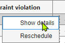
• To view the details of an entry in the Results Table, click the three vertical dots on the right side of the table and select Show details.

  

• To improve efficiency when your objective or nonlinear constraint functions return gradient information or compute in a vectorized manner, set up your problem using Solver Inputs along with Advanced settings.

  

  

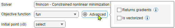
  Currently, fmincon, fminunc, and lsqnonlin can use gradient information, and ga, particleswarm, patternsearch, and surrogateopt can run in a vectorized manner.

Algorithms

Run Mode

The Optimization Explorer app can run in two modes:

• Auto — You specify the maximum time that the app runs, and the app chooses the solvers to try and their order based on the attributes you set and the outcomes of the runs.

• Manual — You specify the solvers, options, and run order.

In both cases, the app stores the results in a table and provides various plots to help visualize the results.

In auto mode:

• Optimization Explorer first runs each solver once using the default options.

• The app then chooses solvers to run using a round robin algorithm. During round robin, the app can select various solver algorithms and adjust some option settings.

• Optimization Explorer runs until it reaches one or more Stopping Conditions.

In manual mode, the app runs all scheduled solvers and then stops.

Configuration Number

As the app runs, it generates configuration numbers that uniquely identify each run. The numbers have the form A.B or A alone, with no decimal point. The decimal point relates to multiple run configurations, such as the same solver and options with different start points (multistart).

• In auto mode, the app does not necessarily perform all runs of multiple run configurations consecutively. For example, configuration 1.20 might run after configuration 2.

• In manual mode, scheduled solver configurations run in the order specified, and configuration numbers increase accordingly.

Stopping Conditions

In auto mode, the following conditions cause the app to stop running:

• The first five solver runs report errors. In this case, try debugging your code for the objective function or nonlinear constraint functions. If the errors are expected outcomes of your code, consider using try-catch statements.

• The first 20 solver runs return exit flag –2 (infeasible). In this case, perhaps the problem is not formulated properly.

• After Optimization Explorer tries all strategies at least once, 50 consecutive solver runs yield insufficient relative improvement in the objective function value. Perhaps a better local solution does not exist, or perhaps the problem is not formulated properly.

• The app finishes all solver configurations, which can occur, for example, when you set the Convex attribute to Yes. In this case, the app runs each applicable configuration once and then stops, because a convex problem has a unique locally optimal objective function value.

• The app reaches the time limit.

Optimization Explorer can continue to run for some time after it reaches a stopping condition, because the app stops solvers using an output function and, therefore, does not interrupt an iteration.

If Optimization Explorer stops because of a stopping condition, you can restart it by clicking Run in the toolstrip.

In manual mode, the app runs all scheduled solvers and then stops.

Version History

Introduced in R2026a