Create Route Planner for Offroad Navigation Using Digital Elevation Data

Since R2024a

Step 1 of 4 in Offroad Navigation for Autonomous Haul Trucks in Open Pit Mine

In this example you will learn how to approximate a road-network using terrain data representing an open-pit mine. Here the terrain is represented as a point cloud that has been stitched together from multiple .LAZ files sourced from the U.S. Geological Survey database. The location chosen for this example is Bingham Canyon, Utah, which contains a copper mine.

Sites like this are interesting because they offer a mix of structured and unstructured terrain, meaning you may want to apply different planning techniques depending on the characteristics of the terrain or problem you want to solve.

"Where we're going, we don't need roads" .... "but they're pretty useful, so let's make some"

The image above shows how switchbacks have been created, leading into the mine. Google Maps does not have any road-network information to offer within the mine, but you can leverage the terrain itself to recapture some of the structure.

Extract Elevation Data from Pointcloud

This example uses a 38 MB point cloud, cleanPC, generated via aerial lidar from the United States Geological Survey [1]. Download the cleanedUSGSPointCloud.zip file from the MathWorks website, then unzip the file using the following:

data = matlab.internal.examples.downloadSupportFile('nav/data/','pitMineClean.mat');

Begin by loading a point cloud that covers our region of interest.

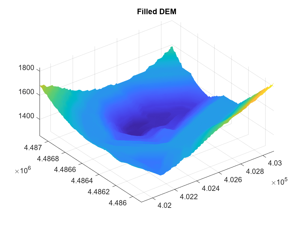
load(data,"cleanPC");

The next step is to convert the raw point cloud to a digital elevation model (dem) using the exampleHelperPc2Grad helper. This function uses pc2dem to sample the initial elevation over the XY limits of the point cloud. The next step is to fill in missing regions of the elevation matrix using scatteredInterpolant, and lastly compute the gradient using griddedInterpolant. The following figures show the original point cloud, followed by the surface that was reconstructed via interpolation.

% Determine the gradient in the point cloud data
res = 1; % cell/meter
[dzdx,dzdy,dem,xlims,ylims,xx,yy] = exampleHelperPc2Grad(cleanPC,res);

% Visualize the open-pit mine with a specified slope limit
figure;
pcshow(cleanPC); 
title("USGS Pointcloud");

figure;
hSurf = surf(xx,yy,dem,EdgeColor="none");
title("Filled DEM");
axis equal;

Identifying Road Boundaries

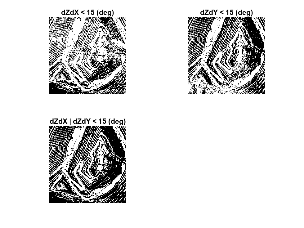
With the slope information identified, separate the terrain into traversable and impassable zones by setting a maximum allowable slope and comparing this against the gradients computed earlier. This gradient mask can be used to restrict our navigable space and does a decent job of highlighting the switchbacks mentioned earlier. Note that slope is just one way you can draw out structure from data representing our environment, others could include semantic-segmentation of an aerial image, or obstacle boundaries generated via sensor data.

% Define maximum allowed slope in radians
slopeMax = 15/180*pi;

% Create masks using slope
maskSlopeX = atan2(abs(dzdx),1/res) < slopeMax;
maskSlopeY = atan2(abs(dzdy),1/res) < slopeMax;

% Binary image with slope masks applied
imSlope = maskSlopeX & maskSlopeY;

% Display off-limit areas whose gradient violates the slope threshold
figure;
f3subplots = exampleHelperComparePlots(gcf,maskSlopeX,maskSlopeY,imSlope);
title(f3subplots(1), "dZdX < " + 180/pi*slopeMax + " (deg)");
title(f3subplots(2), "dZdY < " + 180/pi*slopeMax + " (deg)");
title(f3subplots(3), "dZdX | dZdY < " + 180/pi*slopeMax + " (deg)");

Clean Gradient Mask

Our end goal is to generate a navGraph that can be used to plan high-level routes through our mine, and while the raw gradient mask could be used, the noisy image can lead to disconnected edges, or a large number of paths weaving through tight spaces. To produce a more sensible road-network, you can apply several morphological operations to the mask:

1) imopen (Image Processing Toolbox) is used to fill in small gaps between max-slope regions, producing more consistent off-limit boundaries

% Morphologically filter out narrow passages
se = strel(disk = 4);
imNarrow = imopen(imSlope,se);

2) next imfill (Image Processing Toolbox) is used to eliminate small pockets that would be disconnected from the large free regions in of the map, and therefore useless to our route-planner.

% Fill holes on "exterior" of free road-network region
imHoles = ~imfill(~imNarrow,"holes");

3) then use bwboundaries (Image Processing Toolbox) to identify and remove small pockets of above-average slope. This will make the roads follow the center of major free regions, rather than splitting into multiple paths around small bumps in the terrain.

% Identify any holes that might remain
[B,~,~,~] = bwboundaries(imHoles);
[val,idx] = sort(cellfun(@(x)size(x,1),B));

% Remove interior occupied regions with small boundaries
i = 1;
seedPts = zeros(0,2);
perimeterSizeThreshold = 20; % in cells
while (val(i) < perimeterSizeThreshold)
    ij = B{idx(i)};
    seedPts = [seedPts; ij(1,:)]; %#ok<AGROW>
    i = i + 1;
end

4) lastly, imdilate (Image Processing Toolbox) the remaining mask, solidifying any remaining boundaries

pixelConnectivity = 4;
diskRadius = 3;
imFilled = ~imdilate(bwmorph(~imfill(imHoles,seedPts,pixelConnectivity),"bridge"),ones(diskRadius));

Compare the image after each cleaning operation has been performed:

figure;
f4subplots = exampleHelperComparePlots(gcf,imSlope,imNarrow,imHoles,imFilled);
title(f4subplots(1),"1. Untouched");
title(f4subplots(2),"2. imopen");
title(f4subplots(3),"3. imfill");
title(f4subplots(4),"4. bwboundary-removal");

Convert the Cleaned Image to a Skeleton

Having cleaned up the gradient mask, you can now "skeletonize" the image using bwskel (Image Processing Toolbox), which reduces all free areas in a grayscale image to 1-pixel-wide lines:

%% Skeletonize
rawSkel = bwskel(imFilled,MinBranchLength=75);
se = strel(disk=3);

% Display the skeleton
f5 = figure;
hAx = exampleHelperComparePlots(f5,rawSkel);
hAx.Children.CData = imdilate(hAx.Children.CData,se);

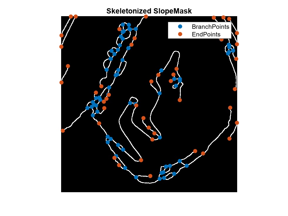
The image is beginning to look like a network of traversable paths, but it lacks connectivity information, so in the next step you will identify all branch and intersection points:

% Compute branch points
branchPts = bwmorph(rawSkel,"branchpoints");

% Compute end points
endPts = bwmorph(rawSkel,"endpoints");
[val,idx] = sort(cellfun(@(x)size(x,1),B));

% Display points atop skeleton
[ib,jb] = ind2sub(size(branchPts),find(flipud(branchPts)'));
[ie,je] = ind2sub(size(branchPts),find(flipud(endPts)'));
hold on;
scatter(hAx, ib(:),jb(:),'o',"filled");
scatter(hAx, ie(:),je(:),'o',"filled");

title(hAx, "Skeletonized SlopeMask");
legend(hAx, {"BranchPoints","EndPoints"});

Extract Edges from Skeleton

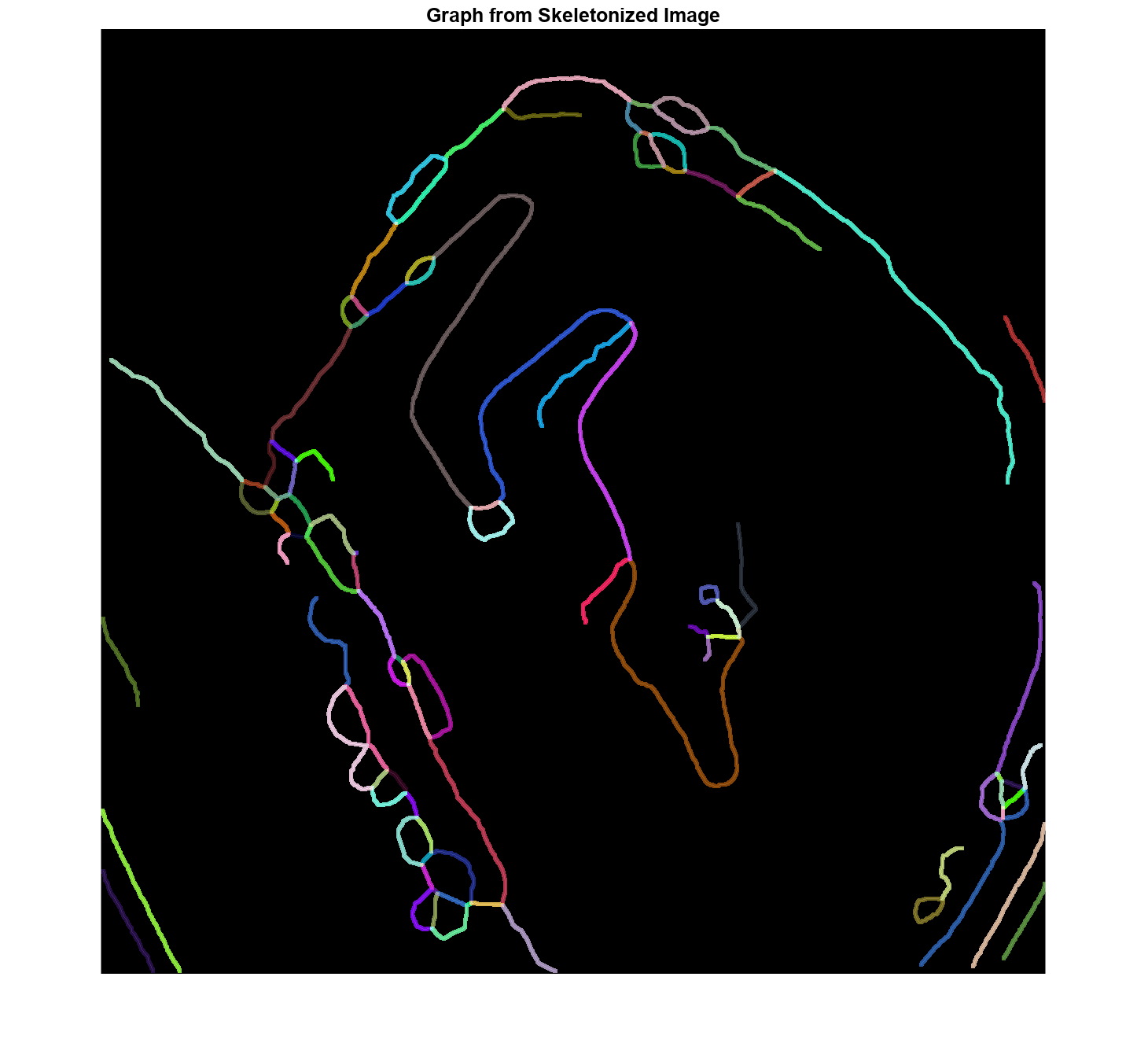
Having reduced our terrain to a skeleton, extract the individual branches from the image. The example helper, exampleHelperSkel2Edges, does this by starting at each end-point and visiting the next free neighbor until another end-point or branch-point is found. The same process is applied to lines originating from the branch-points, with the cells visited along each edge recorded in a corresponding element of a struct-array:

% Crawl the skeleton and build up list of paths
figure;
[pathList,cleanSkel] = exampleHelperSkel2Edges(rawSkel,Visualize=true);

Visualize the set of unique "roads" derived from the terrain:

% Visualize scene
hImg = imshow(cleanSkel);
exampleHelperOverlayPathImage(hImg,pathList,rand(100,3),Radius=3,Frame="ij");
hold on;

Convert Edges to navGraph

The last step is to convert our set of edges to a navGraph, which can be used to return shortest paths between nodes in our road network. The example helper below, exampleHelperPath2GraphData, takes in the list of edges generated by exampleHelperSkel2Edges and converts it to a set of connected nodes, as well as the edges which connect them:

% Use a map to convert our IJ coordinates to XY coordinates
binMap = binaryOccupancyMap(~imSlope,1);
localPathList = pathList;
for i = 1:numel(pathList)
    localPathList(i).Path = grid2local(binMap,pathList(i).Path);
end

% Convert raw path list to graph information
[nodes, edges, edge2pathIdx, cachedPaths] = exampleHelperPath2GraphData(localPathList);

One consideration when creating a route-planner is how "dense" the graph should be. For this reason, exampleHelperPath2GraphData takes an optional second parameter, edgeSize, which dictates how frequently the edges should be subdivided when converting the path list to graph. By default this value is inf, meaning the graph will only be populated using the end-points, leading to a smaller, more efficient search-space.

maxEdgeSize = 25;
[denseNodes, denseEdges, denseEdge2pathIdx, denseCachedPaths] = exampleHelperPath2GraphData(localPathList,maxEdgeSize);

Below you can see the number of edges has increased due to the maxEdgeSize:

disp(size(edges,1));

   226

disp(size(denseEdges,1));

   832

The navGraph also allows for custom edge-costs, so below you will compute the length along the dense path, and store these as Weight in the sparse edges of the graph. Custom cost functions could also consider things like elevation, slope, or even dynamic congestion in cases where the graph is being used to route multiple agents throughout the mine.

% Compute edge weights
numDuplicates = nnz(denseNodes(:,end)~=1);
edgeCosts = exampleHelperDefaultEdgeCost(denseCachedPaths, denseEdge2pathIdx);

Lastly, take advantage of navGraph's ability to store additional meta-data on the edges of the graph. For this particular route planner, you will use this to store Edge2PathIdx - a mapping between the edges in our graph and the set of dense paths in cachedPath. This allows you to fully reconstruct the path between nodes after a route is found.

% Create an astar planner which uses the navGraph constructed using the nodes and edges extracted from the path
stateTable = table(denseNodes,VariableNames={'StateVector'});
linkTable = table(denseEdges, edgeCosts, denseEdge2pathIdx(:), VariableNames={'EndStates','Weight','Edge2PathIdx'});
sparseGraph = navGraph(stateTable,linkTable);

Create A*-Based Route Planner and Find Shortest Path

% Create the planner using the navGraph
planner = plannerAStar(sparseGraph);

% Define a start/goal location slightly away from the nearest node
start = [286.5 423.5];
goal  = [795.5 430.5];

% Find closest node to start and goal location
[dStart,nearStartIdx] = min(vecnorm(denseNodes(:,1:2)-start(1:2),2,2));
[dGoal,nearGoalIdx] = min(vecnorm(denseNodes(:,1:2)-goal(1:2),2,2));

% Plan a route using just the graph
[waypoints, solnInfo] = plan(planner,nearStartIdx,nearGoalIdx);

As mentioned earlier, the graph may be constructed using a sparse representation of the road network, which results in faster planning. The planner produces a sequence of waypoints corresponding to these sparse nodes, so use the Edge2PathIdx metadata to reconstruct the full path:

% Convert path to link-sequence
edgePairs = [solnInfo.PathStateIDs(1:end-1)' solnInfo.PathStateIDs(2:end)'];
linkID = findlink(planner.Graph,edgePairs);
networkPath = vertcat(denseCachedPaths(planner.Graph.Links.Edge2PathIdx(linkID)).Path);

Lastly, visualize the shortest path through the copper mine:

Visualize Scene

figure;
hIm = show(binMap);
cmap = colormap("spring");
exampleHelperOverlayPathImage(hIm,pathList,cmap(randi(size(cmap,1),100),:),Radius=0);
hold on;
gHandle = show(planner.Graph);
gHandle.XData = planner.Graph.States.StateVector(:,1); 
gHandle.YData = planner.Graph.States.StateVector(:,2);
exampleHelperPlotLines(networkPath,{"LineWidth",4});
startSpec = plannerLineSpec.start(MarkerEdgeColor="red",MarkerFaceColor="red");
plot(start(1),start(2),startSpec{:})
goalSpec = plannerLineSpec.goal(MarkerEdgeColor="green",MarkerFaceColor="green");
plot(goal(1),goal(2),goalSpec{:})
legendStrings = ["navGraph","networkPath","Start","Goal"];
legend(legendStrings);

Conclusion

In this example you learned how to infer structure from USGS-sourced terrain data and used this structure to generate a route planner. You began by extracting the gradient from a digital elevation model, and then used morphological operations on a slope-masked image to identify the free and off-limit regions. The remaining free-space was then skeletonized, with the remaining edges forming the boundaries of an implicit Voronoi field. Lastly, you saw how the skeleton can be converted to a navGraph and used as an informal route planner.

In Create Terrain-Aware Global Planners for Offroad Navigation, you will develop a utility that can generate paths onto the graph while adhering to a vehicle's non-holonomic constraints and learn how to create a terrain-aware planner for navigating unstructured regions of our mine using plannerHybridAStar.

References

1. cleanPC compiled from National Map 3DEP Downloadable Data Collection courtesy of the U.S. Geological Survey