scatteredInterpolant

Interpolate 2-D or 3-D scattered data

Description

Use scatteredInterpolant to perform interpolation on a 2-D or 3-D data set of scattered data. scatteredInterpolant returns the interpolant F for the given data set. You can evaluate F at a set of query points, such as (xq,yq) in 2-D, to produce interpolated values vq = F(xq,yq).

Use griddedInterpolant to perform interpolation with gridded data.

Creation

Syntax

F = scatteredInterpolant

F = scatteredInterpolant(x,y,v)

F = scatteredInterpolant(x,y,z,v)

F = scatteredInterpolant(P,v)

F = scatteredInterpolant(___,Method)

F = scatteredInterpolant(___,Method,ExtrapolationMethod)

Description

F = scatteredInterpolant creates an empty scattered data interpolant object.

F = scatteredInterpolant(x,y,v) creates an interpolant that fits a surface of the form v = F(x,y). Vectors x and y specify the (x,y) coordinates of the sample points. v contains the sample values associated with the points (x,y).

F = scatteredInterpolant(x,y,z,v) creates a 3-D interpolant of the form v = F(x,y,z).

F = scatteredInterpolant(P,v) specifies the coordinates of the sample points as an array. The rows of P contain the (x, y) or (x, y, z) coordinates for the values in v.

F = scatteredInterpolant(___,Method) specifies an interpolation method 'nearest', 'linear', or 'natural' as the last input argument in any of the first three syntaxes.

F = scatteredInterpolant(___,Method,ExtrapolationMethod) specifies both the interpolation and extrapolation methods. Pass Method and ExtrapolationMethod together as the last two input arguments in any of the first three syntaxes.

Input Arguments

x, y, z — Sample points

column vectors

Sample points, specified as column vectors with the same number of rows as v. The sample points should be unique. However, if the sample points contain duplicates, scatteredInterpolant displays a warning and merges the duplicates into a single point.

The x, y, and z arguments set the value of the Points property of the scatteredInterpolant object.

Data Types: double

P — Sample points array

matrix

Sample points array, specified as an m-by-n matrix, where m is the number of points and n is the dimension of the space where the points reside. Each row of P contains the (x, y) or (x, y, z) coordinates of a sample point. The sample points should be unique. However, if the sample points contain duplicates, scatteredInterpolant displays a warning and merges the duplicates into a single point.

This argument sets the Points property of the scatteredInterpolant object.

Data Types: double

v — Function values at sample points

vector | matrix

Function values at sample points, specified as a vector or matrix. For 2-D data, v = F(x,y). For 3-D data, v = F(x,y,z).

• To interpolate using a single set of values, specify v as a vector, where the number of rows is the same as the number of sample points.

• To interpolate using multiple sets of values, specify v as a matrix, where the number of rows is the same as the number of sample points. Each column in v represents the values of a different function at the sample points. For example, if x and y are column vectors with 10 elements, you can specify v as a 10-by-4 matrix to interpolate using four different sets of values.

scatteredInterpolant does not ignore NaN values in v, so interpolation results near those sample points are also NaN.

This argument sets the Values property of the scatteredInterpolant object.

Data Types: double

Method — Interpolation method

'linear' (default) | 'nearest' | 'natural'

Interpolation method, specified as one of these options.

Method	Description	Continuity
'linear' (default)	Linear interpolation	C0
'nearest'	Nearest neighbor interpolation	Discontinuous
'natural'	Natural neighbor interpolation	C1 (except at sample points)

This argument sets the Method property of the scatteredInterpolant object.

ExtrapolationMethod — Extrapolation method

'linear' | 'nearest' | 'boundary' | 'none'

Extrapolation method, specified as one of these options.

Extrapolation Method	Description
'linear'	Linear extrapolation based on boundary gradients. This method is the default when Method is 'linear' or 'natural'.
'nearest'	Nearest neighbor extrapolation. This method evaluates to the value of the nearest neighbor. This method is the default when Method is 'nearest'.
'boundary' (since R2024a)	Boundary extrapolation. This method extends the values on the interpolation boundary into the extrapolation domain.
'none'	No extrapolation. Any queries outside the convex hull of Points return NaN.

This argument sets the ExtrapolationMethod property of the scatteredInterpolant object.

Properties

Points — Sample points

matrix

Sample points, specified as a matrix. The size of the matrix is m-by-2 or m-by-3 to represent m points in 2-D or 3-D space. Each row of Points contains the (x, y) or (x, y, z) coordinates of a unique sample point. The rows in Points correspond to the function values in Values.

Data Types: double

Values — Function values at sample points

vector | matrix

Function values at sample points, specified as a vector or matrix. This property is set by the v input argument.

Data Types: double

Method — Interpolation method

'linear' (default) | 'nearest' | 'natural'

Interpolation method, specified as 'linear','nearest' , or 'natural'. See Method for descriptions of these methods.

ExtrapolationMethod — Extrapolation method

'linear' | 'nearest' | 'boundary' | 'none'

Extrapolation method, specified as 'linear', 'nearest', 'boundary' (since R2024a), or 'none'. See ExtrapolationMethod for descriptions of these methods.

Usage

Syntax

Vq = F(Pq)

Vq = F(Xq,Yq)

Vq = F(Xq,Yq,Zq)

Vq = F({xq,yq})

Vq = F({xq,yq,zq})

Description

Use scatteredInterpolant to create the interpolant, F. Then you can evaluate F at specific points using any of the following syntaxes.

Vq = F(Pq) evaluates F at the query points in the matrix Pq. Each row in Pq contains the coordinates of a query point.

Vq = F(Xq,Yq) and Vq = F(Xq,Yq,Zq) specify query points as two or three arrays of equal size. F treats the query points as column vectors, for example, Xq(:).

• If the Values property of F is a column vector representing one set of values at the sample points, then Vq is the same size as the query points.

• If the Values property of F is a matrix representing multiple sets of values at the sample points, then Vq is a matrix, and each column represents a different set of values at the query points.

Vq = F({xq,yq}) and Vq = F({xq,yq,zq}) specify query points as grid vectors. Use this syntax to conserve memory when you want to query a large grid of points.

Examples

2-D Interpolation

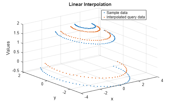
Define some sample points and calculate the value of a trigonometric function at those locations. These points are the sample values for the interpolant.

t = linspace(3/4*pi,2*pi,50)';
x = [3*cos(t); 2*cos(t); 0.7*cos(t)];
y = [3*sin(t); 2*sin(t); 0.7*sin(t)];
v = repelem([-0.5; 1.5; 2],length(t));

Create the interpolant.

F = scatteredInterpolant(x,y,v);

Evaluate the interpolant at query locations (xq,yq).

tq = linspace(3/4*pi+0.2,2*pi-0.2,40)';
xq = [2.8*cos(tq); 1.7*cos(tq); cos(tq)];
yq = [2.8*sin(tq); 1.7*sin(tq); sin(tq)];
vq = F(xq,yq);

Plot the result.

plot3(x,y,v,'.',xq,yq,vq,'.'), grid on
title('Linear Interpolation')
xlabel('x'), ylabel('y'), zlabel('Values')
legend('Sample data','Interpolated query data','Location','Best')

3-D Interpolation

Create an interpolant for a set of scattered sample points, then evaluate the interpolant at a set of 3-D query points.

Define 200 random points and sample a trigonometric function. These points are the sample values for the interpolant.

rng default;
P = -2.5 + 5*rand([200 3]);
v = sin(P(:,1).^2 + P(:,2).^2 + P(:,3).^2)./(P(:,1).^2+P(:,2).^2+P(:,3).^2);

Create the interpolant.

F = scatteredInterpolant(P,v);

Evaluate the interpolant at query locations (xq,yq,zq).

[xq,yq,zq] = meshgrid(-2:0.25:2);
vq = F(xq,yq,zq);

Plot slices of the result.

xslice = [-.5,1,2]; 
yslice = [0,2]; 
zslice = [-2,0];
slice(xq,yq,zq,vq,xslice,yslice,zslice)

Replacement of Sample Values

Replace the elements in the Values property when you want to change the values at the sample points. You get immediate results when you evaluate the new interpolant because the original triangulation does not change.

Create 50 random points and sample an exponential function. These points are the sample values for the interpolant.

rng('default')
x = -2.5 + 5*rand([50 1]);
y = -2.5 + 5*rand([50 1]);
v = x.*exp(-x.^2-y.^2);

Create the interpolant.

F = scatteredInterpolant(x,y,v)

F = 
  scatteredInterpolant with properties:

                 Points: [50×2 double]
                 Values: [50×1 double]
                 Method: 'linear'
    ExtrapolationMethod: 'linear'

Evaluate the interpolant at (1.40,1.90).

F(1.40,1.90)

ans = 
0.0069

Change the interpolant sample values and reevaluate the interpolant at the same point.

vnew = x.^2 + y.^2;
F.Values = vnew;
F(1.40,1.90)

ans = 
5.6491

Eliminate Duplicate Sample Points

Use groupsummary to eliminate duplicate sample points and control how they are combined prior to calling scatteredInterpolant.

Create a 200-by-3 matrix of sample point locations. Add duplicate points in the last five rows.

P = -2.5 + 5*rand(200,3);
P(197:200,:) = repmat(P(196,:),4,1);

Create a vector of random values at the sample points.

V = rand(size(P,1),1);

If you attempt to use scatteredInterpolant with duplicate sample points, it throws a warning and averages the corresponding values in V to produce a single unique point. However, you can use groupsummary to eliminate the duplicate points prior to creating the interpolant. This is particularly useful if you want to combine the duplicate points using a method other than averaging.

Use groupsummary to eliminate the duplicate sample points and preserve the maximum value in V at the duplicate sample point location. Specify the sample points matrix as the grouping variable and the corresponding values as the data.

[V_unique,P_unique] = groupsummary(V,P,@max);

Since the grouping variable has three columns, groupsummary returns the unique groups P_unique as a cell array. Convert the cell array back into a matrix.

P_unique = [P_unique{:}];

Create the interpolant. Since the sample points are now unique, scatteredInterpolant does not throw a warning.

I = scatteredInterpolant(P_unique,V_unique);

Compare Scattered Data Interpolation Methods

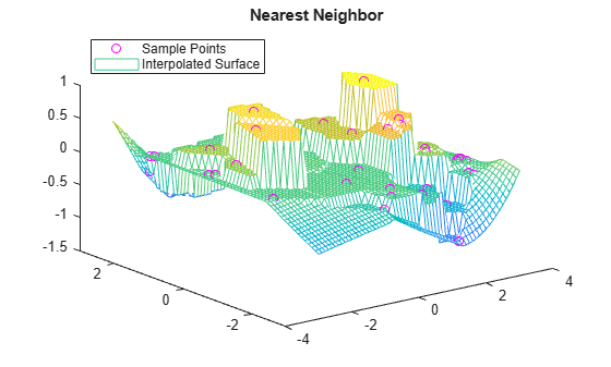
Compare the results of several different interpolation algorithms offered by scatteredInterpolant.

Create a sample data set of 50 scattered points. The number of points is artificially small to highlight the differences between the interpolation methods.

x = -3 + 6*rand(50,1);
y = -3 + 6*rand(50,1);
v = sin(x).^4 .* cos(y);

Create the interpolant and a grid of query points.

F = scatteredInterpolant(x,y,v);
[xq,yq] = meshgrid(-3:0.1:3);

Plot the results using the 'nearest', 'linear', and 'natural' methods. Each time the interpolation method changes, you need to requery the interpolant to get the updated results.

F.Method = 'nearest';
vq1 = F(xq,yq);
plot3(x,y,v,'mo')
hold on
mesh(xq,yq,vq1)
title('Nearest Neighbor')
legend('Sample Points','Interpolated Surface','Location','NorthWest')

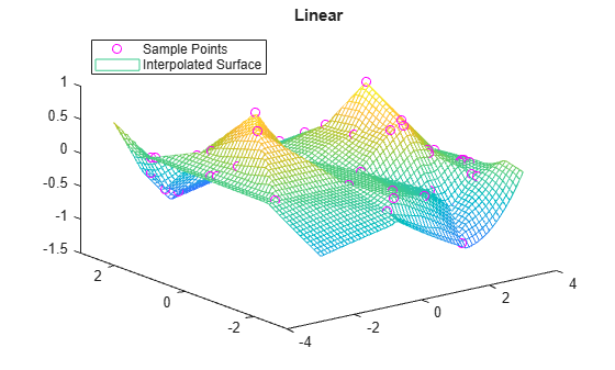
F.Method = 'linear';
vq2 = F(xq,yq);
figure
plot3(x,y,v,'mo')
hold on
mesh(xq,yq,vq2)
title('Linear')
legend('Sample Points','Interpolated Surface','Location','NorthWest')

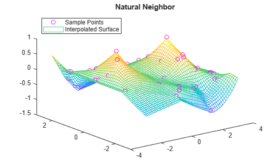
F.Method = 'natural';
vq3 = F(xq,yq);
figure
plot3(x,y,v,'mo')
hold on
mesh(xq,yq,vq3)
title('Natural Neighbor')
legend('Sample Points','Interpolated Surface','Location','NorthWest')

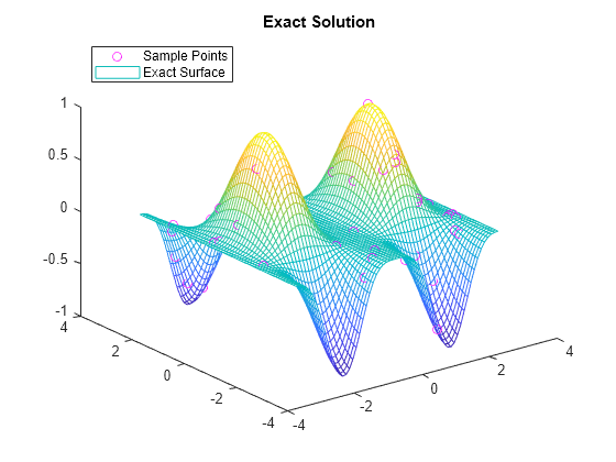
Plot the exact solution.

figure
plot3(x,y,v,'mo')
hold on
mesh(xq,yq,sin(xq).^4 .* cos(yq))
title('Exact Solution')
legend('Sample Points','Exact Surface','Location','NorthWest')

Compare Scattered Data Extrapolation Methods

Since R2024a

Compare the results of several different extrapolation methods offered by scatteredInterpolant.

Create a sample data set of 50 scattered points, and calculate the value of a trigonometric function at those locations. These points are the sample values for the interpolant.

rng default
x = -3 + 6*rand(50,1);
y = -3 + 6*rand(50,1);
v = sin(x).^4 .* cos(y);

Create the interpolant.

F = scatteredInterpolant(x,y,v)

F = 
  scatteredInterpolant with properties:

                 Points: [50×2 double]
                 Values: [50×1 double]
                 Method: 'linear'
    ExtrapolationMethod: 'linear'

Compute the boundary of the input data.

C = convhull(x,y);
xc = [x(C); x(C(1))];
yc = [y(C); y(C(1))];
vc = [v(C); v(C(1))];

Evaluate the interpolant at query locations (xq,yq) using linear extrapolation based on boundary gradients. Then, plot the result of the interpolation and extrapolation.

[xq,yq] = meshgrid(-4:0.1:4);
vq1 = F(xq,yq);

surf(xq,yq,vq1,FaceAlpha=0.5,DisplayName="Interpolation + extrapolation result",EdgeColor=[100 100 100]./256,FaceColor="interp")
hold on
plot3(x,y,v,"black.",MarkerSize=20,DisplayName="Sample points")
plot3(xc,yc,vc,"magenta-",LineWidth=3,DisplayName="Interpolation-extrapolation boundary")
title("Linear interpolation + linear extrapolation")
legend(Location="NorthEast")
zlim([-2.8 1.3])
colorbar
colormap jet
clim([-2.8 1.3])
view([-183.69 21.20])
hold off

Modify the interpolant to use nearest neighbor extrapolation, and evaluate and visualize the interpolant.

F.ExtrapolationMethod = "nearest";
vq2 = F(xq,yq);

surf(xq,yq,vq2,FaceAlpha=0.5,DisplayName="Interpolation + extrapolation result",EdgeColor=[100 100 100]./256,FaceColor="interp")
hold on
plot3(x,y,v,"black.",MarkerSize=20,DisplayName="Sample points")
plot3(xc,yc,vc,"magenta-",LineWidth=3,DisplayName="Interpolation-extrapolation boundary")
title("Linear interpolation + Nearest extrapolation")
legend(Location="NorthEast")
zlim([-2.8 1.3])
colorbar
colormap jet
clim([-2.8 1.3])
view([-183.69 21.20])
hold off

Modify the interpolant to extend the interpolation boundary into the extrapolation domain, and evaluate and visualize the interpolant.

F.ExtrapolationMethod = "boundary";
vq3 = F(xq,yq);

surf(xq,yq,vq3,FaceAlpha=0.5,DisplayName="Interpolation + extrapolation result",EdgeColor=[100 100 100]./256,FaceColor="interp")
hold on
plot3(x,y,v,"black.",MarkerSize=20,DisplayName="Sample points")
plot3(xc,yc,vc,"magenta-",LineWidth=3,DisplayName="Interpolation-extrapolation boundary")
title("Linear interpolation + Boundary extrapolation")
legend(Location="NorthEast")
zlim([-2.8 1.3])
colorbar
colormap jet
clim([-2.8 1.3])
view([-183.69 21.20])
hold off

Compare the extrapolation methods by examining the plotted results. Boundary extrapolation preserves continuity between the interpolation and extrapolation domain, while nearest neighbor extrapolation can be discontinuous along the boundary. Boundary extrapolation does not produce extreme values in the extrapolation domain, while linear extrapolation can produce extreme values.

Interpolate Multiple Sets of Values at Query Points

Since R2023b

Interpolate multiple data sets at the same query points.

Create a sample data set with 50 scattered points represented by sample point vectors x and y.

rng("default")
x = -3 + 6*rand(50,1);
y = -3 + 6*rand(50,1);

To interpolate multiple data sets, create a matrix where each column represents the values of a different function at the sample points.

s1 = sin(x).^4 .* cos(y);
s2 = sin(x) + cos(y);
s3 = x + y;
s4 = x.^2 + y;
v = [s1 s2 s3 s4];

Create query point vectors, which indicate the locations to perform interpolation for each set of values in v.

xq = -3:0.1:3;
yq = -3:0.1:3;

Create the interpolant F.

F = scatteredInterpolant(x,y,v)

F = 
  scatteredInterpolant with properties:

                 Points: [50×2 double]
                 Values: [50×4 double]
                 Method: 'linear'
    ExtrapolationMethod: 'linear'

Evaluate the interpolant at the query locations. Each page of Vq contains the interpolated values for the corresponding data set in v.

Vq = F({xq,yq});
size(Vq)

ans = 1×3

    61    61     4

Plot the interpolated values for each data set.

tiledlayout(2,2)
nexttile
plot3(x,y,v(:,1),'mo')
hold on
mesh(xq,yq,Vq(:,:,1)')
title("sin(x).^4 .* cos(y)")

nexttile
plot3(x,y,v(:,2),'mo')
hold on
mesh(xq,yq,Vq(:,:,2)')
title("sin(x) + cos(y)")

nexttile
plot3(x,y,v(:,3),'mo')
hold on
mesh(xq,yq,Vq(:,:,3)')
title("x + y")

nexttile
plot3(x,y,v(:,4),'mo')
hold on
mesh(xq,yq,Vq(:,:,4)')
title("x.^2 + y")

lg = legend("Sample Points","Interpolated Surface");
lg.Layout.Tile = "north";

More About

Interpolant

Interpolating function that you can evaluate at query points.

Gridded Data

A set of points that are axis-aligned and ordered.

Scattered Data

A set of points that have no structure among their relative locations.

Full Grid

A grid represented as a set of arrays. For example, you can create a full grid using ndgrid.

Grid Vectors

A set of vectors that serve as a compact representation of a grid in ndgrid format.

For example, [X,Y] = ndgrid(xg,yg) returns a full grid in the matrices X and Y. You can represent the same grid using the grid vectors xg and yg.

Tips

• It is quicker to evaluate a scatteredInterpolant object F at many different sets of query points than it is to compute the interpolations separately using the functions griddata or griddatan. For example:

  % Fast to create interpolant F and evaluate multiple times
  F = scatteredInterpolant(X,Y,V)
  v1 = F(Xq1,Yq1)
  v2 = F(Xq2,Yq2)
  
  % Slower to compute interpolations separately using griddata
  v1 = griddata(X,Y,V,Xq1,Yq1)
  v2 = griddata(X,Y,V,Xq2,Yq2)
  

• To change the interpolation sample values or interpolation method, it is more efficient to update the properties of the interpolant object F than it is to create a new scatteredInterpolant object. When you update Values or Method, the underlying Delaunay triangulation of the input data does not change, so you can compute new results quickly.

• Scattered data interpolation with scatteredInterpolant uses a Delaunay triangulation of the data, so interpolation can be sensitive to scaling issues in the sample points x, y, z, or P. When scaling issues occur, you can use normalize to rescale the data and improve the results. See Normalize Data with Differing Magnitudes for more information.

Algorithms

scatteredInterpolant uses a Delaunay triangulation of the scattered sample points to perform interpolation [1].

References

[1] Amidror, Isaac. “Scattered data interpolation methods for electronic imaging systems: a survey.” Journal of Electronic Imaging. Vol. 11, No. 2, April 2002, pp. 157–176.

Extended Capabilities

C/C++ Code Generation

Generate C and C++ code using MATLAB® Coder™. (since R2024b)

Usage notes and limitations:

• Query points and input data must be two-dimensional.

• Method and ExtrapolationMethod must be constants (known values when code is generated).

• Empty interpolant objects are not supported for code generation.

• If the sample values or query points contain Inf or -Inf, the output of the generated code might not match the output in MATLAB^®.

• In certain cases, the behavior of the generated code might differ from MATLAB. For code generation, scatteredInterpolant is based on Qhull. For more information, see http://www.qhull.org/. For copyright information, see http://www.qhull.org/COPYING.txt.

Thread-Based Environment

Run code in the background using MATLAB® backgroundPool or accelerate code with Parallel Computing Toolbox™ ThreadPool.

This function fully supports thread-based environments. For more information, see Run MATLAB Functions in Thread-Based Environment.

Version History

Introduced in R2013a

R2024a: Extrapolate using boundary values

Specify the 'boundary' extrapolation method to extend the values on the interpolation boundary into the extrapolation domain. This method mitigates extreme extrapolation values and maintains continuity between the extrapolation and interpolation domains.

R2023b: Interpolate multiple data sets simultaneously

Specify the sample values v as a matrix to interpolate multiple data sets on the same grid at the same query points. Each column in v represents the values of a different function at the sample points. For example, if x and y are column vectors with 10 elements, you can specify v as a 10-by-4 matrix to interpolate using four different sets of values.

Previously, you could specify v only as a vector, and multivalued interpolation was available only for griddedInterpolant.