Validate Nonlinear ARX Models
After estimating a nonlinear ARX model for your system, you can validate whether it reproduces the system behavior within acceptable bounds. You can validate your model in different ways. It is recommended that you use separate data sets for estimating and validating your model. If the validation indicates low confidence in the estimation, then see Troubleshooting Model Estimation for next steps. For general information about validating models, see Model Validation.
Compare Model Output to Measured Output
Plot simulated or predicted model output and measured output
data for comparison, and compute best fit values. At the command line,
use compare command. You can
also use sim and predict to simulate and predict model
response. For information about plotting simulated and predicted output
in the app, see Simulation and Prediction in the App.
Check Iterative Search Termination Conditions
The estimation report that is generated after model estimation lists the reason the software terminated the estimation. For example, suppose that the report indicates that the estimation reached the maximum number of iterations. You can try repeating the estimation by specifying a larger value for the maximum number of iterations. For information about how to configure the maximum number of iterations and other estimation options, see Specify Estimation Options for Nonlinear ARX Models.
To view the estimation report in the app, after model estimation is complete, view the
Estimation Report area of the Estimate
tab. At the command line, use M.Report.Termination to display the
estimation termination conditions, where M is the estimated
Nonlinear ARX model. For example, check the
M.Report.Termination.WhyStop field that describes why the
estimation was stopped.
For more information about the estimation report, see Estimation Report.
Check the Final Prediction Error and Loss Function Values
You can compare the performance of several estimated models by comparing the final prediction error and loss function values that are shown in the estimation report.
To view these values for an estimated model M at
the command line, use the M.Report.Fit.FPE (final
prediction error) and M.Report.Fit.LossFcn (value
of loss function at estimation termination) properties. Smaller values
typically indicate better performance. However, M.Report.Fit.FPE values
can be unreliable when the model contains many parameters relative
to the estimation data size. Use these indicators with other validation
techniques to draw reliable conclusions.
Perform Residual Analysis
Residuals are differences between the model output and the measured output. Thus, residuals represent the portion of the output not explained by the model. You can analyze the residuals using techniques such as the whiteness test and the independence test. For more information about these tests, see What Is Residual Analysis?.
At the command line, use resid to
compute, plot, and analyze the residuals. To plot residuals in the
app, see How to Plot Residuals in the App.
Examine Nonlinear ARX Plots
A nonlinear ARX plot displays the evaluated model nonlinearity for a chosen
model output as a function of one or two model regressors. For a model M,
the model nonlinearity (M.Nonlinearity) is a nonlinearity estimator
function, such as idWaveletNetwork, idSigmoidNetwork, or idTreePartition, that uses model regressors as
its inputs.
To understand what is plotted, suppose that {r1,r2,…,rN} are
the N regressors used by a nonlinear ARX model M with
nonlinearity nl corresponding to a model output.
You can use getreg(M) to view these regressors.
The expression Nonlin = evaluate(nl,[v1,v2,...,vN]) returns
the model output for given values of these regressors, that is, r1 = v1, r2 = v2,
..., rN = vN. For plotting the
nonlinearities, you select one or two of the N regressors,
for example, rsub = {r1,r4}. The software varies
the values of these regressors in a specified range, while fixing
the value of the remaining regressors, and generates the plot of Nonlin vs. rsub.
By default, the software sets the values of the remaining fixed regressors
to their estimated means, but you can change these values. The regressor
means are stored in the Nonlinearity.Parameters.RegressorMean property
of the model.
Examining a nonlinear ARX plot can help you gain insight into which regressors have the strongest effect on the model output. Understanding the relative importance of the regressors on the output can help you decide which regressors to include in the nonlinear function for that output. If the shape of the plot looks like a plane for all the chosen regressor values, then the model is probably linear in those regressors. In this case, you can remove the corresponding regressors from nonlinear block, and repeat the estimation.
Furthermore, you can create several nonlinear models for the same data using different
nonlinearity estimators, such a idWaveletNetwork network and
idTreePartition, and then compare the nonlinear surfaces of these
models. Agreement between plots for various models increases the confidence that these
nonlinear models capture the true dynamics of the system.
Creating a Nonlinear ARX Plot
To create a nonlinear ARX plot in the System Identification app, select the Nonlinear ARX check box in the Model Views area. To include or exclude a model on the plot, click the corresponding model icon in the app. For general information about creating and working with plots in the app, see Working with Plots.
At the command line, after you have estimated a nonlinear ARX model M, use
nlarxPlot to view the shape of
the nonlinearity.
plot(M)
You can use additional plot arguments to
specify the following information:
Include multiple nonlinear ARX models on the plot.
Configure the regressor values for computing the nonlinearity values.
Configuring a Nonlinear ARX Plot
To configure the nonlinear ARX plot:
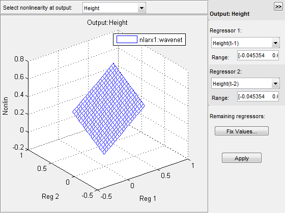
Select the output channel in the Select nonlinearity at output drop-down list. The nonlinearity values that correspond to the selected output channel are displayed.
Select Regressor 1 from the list of available regressors. In the Range field, enter the range of values to include on the plot for this regressor. The regressor values are plotted on the Reg1 axis of the plot.
If the regressor selection options are not visible, click
 to expand the Nonlinear
ARX Model Plot window.
to expand the Nonlinear
ARX Model Plot window.Specify Regressor 2 as one of the following options:
To display three axes on the plot, select Regressor 2. In the Range field, enter the range of values to include on the plot for this regressor. The regressor values are plotted on the Reg2 axis of the plot.
To display only two axes, select
<none>in the Regressor 2 list.
Fix the values of the regressors that are not displayed by clicking Fix Values. In the Fix Regressor Values dialog box, double-click the Value cell to edit the constant value of the corresponding regressor. The default values are determined during model estimation. Click OK.
If you generate the nonlinear ARX plot in the app, you can perform the following additional tasks:
| Action | Procedure |
|---|---|
| Change the grid spacing of the regressors along each axis. | In the plot window, select Options > Set number of samples, and enter the number of samples to use for each regressor. Click Apply and then Close. For example, if the number of samples is 20, each regressor variable contains 20 points in its specified range. For a 3-D plots, this results in evaluating the nonlinearity at 20 x 20 = 400 points. |
| Change axis limits. | Select Options > Set axis limits to open the Axis Limits dialog box, and edit the limits. Click Apply. |
| Hide or show the plot legend. | Select Style > Legend. Select this option again to show the legend. |
|
Rotate in three dimensions. Note Available only when you have selected two regressors as independent variables. | Select Style > Rotate 3D and drag the axes on the plot to a new orientation. To disable three-dimensional rotation, select Style > Rotate 3D again. |
See Also
compare | sim | resid | predict