Generate NARMAX Models

This example uses:

This example shows how to generate NARMAX models using the available model structures and their training algorithms by preparing a finite-horizon prediction algorithm. The available model structures include nonlinear ARX, grey-box, and neural state-space models. For more information on the model structures, see NARMAX Model Identification.

Consider a scalar time series, y, that is observed for 1000 seconds at an interval of one second. The values of y are influenced by an exogenous input, u. The observations of u and y are recorded in a timetable, TT. In the standard system identification terminology, TT represents the observations of a single-input single-output (SISO) system.

Load the timetable.

load NARMAXExampleData TT
stackedplot(TT)

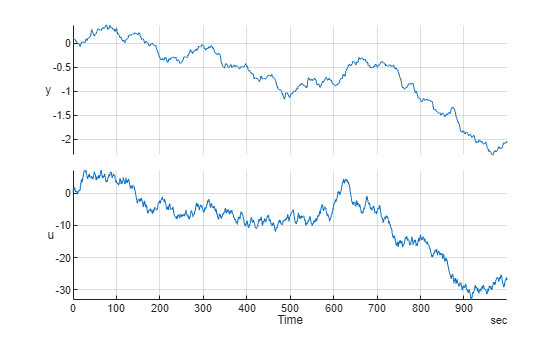
Figure contains an object of type stackedplot.

grid on

Prepare training and validation data. Use the first half of the data for all model training exercises and the second half for validation of the results.

TrainData = TT(1:500,:); 
TrainData.Properties.Description = "Training Data";
ValidateData = TT(501:end,:);
ValidateData.Properties.Description = "Validation Data";
wrn = warning('off','Ident:estimation:NparGTNsamp');
cl = onCleanup(@()warning(wrn));

Linear ARMAX Model

First, set a reference by fitting a linear ARMAX model to the data. To choose a model order such that the model best fits the data, call the ssest command with orders from 1 to 10.

ssest(TT,1:10)

ans =
  Continuous-time identified state-space model:
      dx/dt = A x(t) + B u(t) + K e(t)
       y(t) = C x(t) + D u(t) + e(t)
 
  A = 
             x1        x2
   x1  -0.01522   -0.8502
   x2   -0.1401    -8.357
 
  B = 
             y
   x1  0.09112
   x2   0.8983
 
  C = 
          x1      x2
   u   -97.8  -14.25
 
  D = 
      y
   u  0
 
  K = 
              u
   x1  -0.02206
   x2  -0.05002
 
Parameterization:
   FREE form (all coefficients in A, B, C free).
   Feedthrough: none
   Disturbance component: estimate
   Number of free coefficients: 10
   Use "idssdata", "getpvec", "getcov" for parameters and their uncertainties.

Status:                                          
Estimated using SSEST on time domain data "TT".  
Fit to estimation data: 79.42% (prediction focus)
FPE: 4.114, MSE: 4.065                           
 
Model Properties

You can see that a model order of two gives the best fit. Using this knowledge, set na=nb=nc=2 and nk=1 to create the linear ARMAX model using armax. Setting nk=1 indicates that you assume there is no feedthrough.

na = 2;
nb = 2;
nc = 2;
nk = 1;
sysARMAX = armax(TrainData,[na nb nc nk],InputName="u")

sysARMAX =
Discrete-time ARMAX model: A(z)y(t) = B(z)u(t) + C(z)e(t)
  A(z) = 1 - 0.4184 z^-1 - 0.5859 z^-2                   
                                                         
  B(z) = 0.001209 z^-1 - 0.0009946 z^-2                  
                                                         
  C(z) = 1 + 1.908 z^-1 + 0.9852 z^-2                    
                                                         
Sample time: 1 seconds
  
Parameterization:
   Polynomial orders:   na=2   nb=2   nc=2   nk=1
   Number of free coefficients: 6
   Use "polydata", "getpvec", "getcov" for parameters and their uncertainties.

Status:                                               
Estimated using ARMAX on time domain data "TrainData".
Fit to estimation data: 97.23% (prediction focus)     
FPE: 0.0001116, MSE: 0.0001081                        
 
Model Properties

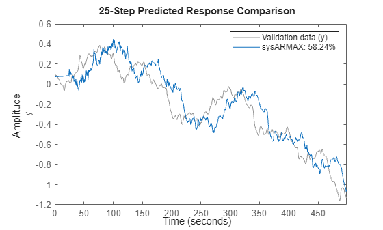
Check the model performance on training data by its ability to forecast 25 steps into the future using compare.

compare(TrainData,sysARMAX,25)

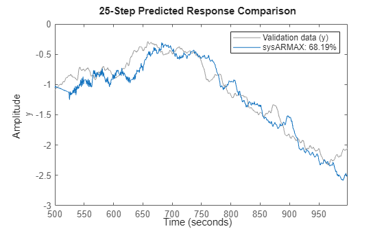
Figure contains an axes object. The axes object with ylabel y contains 2 objects of type line. These objects represent Validation data (y), sysARMAX: 58.24%.

Check the model performance on validation data.

clf
compare(ValidateData,sysARMAX,25)

Figure contains an axes object. The axes object with ylabel y contains 2 objects of type line. These objects represent Validation data (y), sysARMAX: 68.19%.

NARMAX Models with Linear and Additive Moving Average Term

System Identification Toolbox™ supports estimation of NARX models but not the NARMAX models. However, this example shows how to obtain a NARMAX model using the nlarx command together with a grey-box (nlgreyest) based refinement step.

To create a NARMAX model with additive moving average terms:

Fit a NARX model to the data using the nlarx command.
Compute the model residuals using the pe or resid command.
Fit a linear moving average (MA) model to the residuals using the armax command with na = 0, nc = MA order.
Combine the NARX model with the linear MA model using the grey-box modeling approach (see idnlgrey and nlgreyest). To improve the fit to the data, refine the free coefficients of the resulting grey-box model.

Nonlinear ARX

To fit a NARX model to the data, you need two pieces of information: the model regressors and the nature of the function that maps the regressors to the predicted response.

Use the linear regressors, $y (k - 1), y (k - 2), u (k - 1), u (k - 2), u (k - 3)$ . This choice is consistent with the model orders used for the linear model sysARMAX.
Use two hidden layers with five sigmoid activations each for the nonlinear function that maps the regressors to the output.

The parameters of this model are the various weights and biases used by the fully connected layers of the nonlinear (neural network) function.

Create the regressor functions using linearRegressor.

Reg = linearRegressor(["y","u"],{1:2, 1:3});  
getreg(Reg)

ans = 5×1 string
    "y(t-1)"
    "y(t-2)"
    "u(t-1)"
    "u(t-2)"
    "u(t-3)"

Create the nonlinear function, which is a two-layer neural network with sigmoid activations, using idNeuralNetwork.

NL = idNeuralNetwork([5 5],"sigmoid",NetworkType="RegressionNeuralNetwork")

NL = 
Multi-Layer Neural Network

 Nonlinear Function: Uninitialized regression neural network
         Contains 2 hidden layers using "sigmoid" activations.
         (uses Statistics and Machine Learning Toolbox)
 Linear Function: uninitialized
 Output Offset: uninitialized

              Network: 'Regression neural network parameters'
            LinearFcn: 'Linear function parameters'
               Offset: 'Offset parameters'
    EstimationOptions: [1×1 struct]

Specify estimation options and create a nonlinear ARX model by training it in closed-loop, that is, by minimizing the simulation errors.

opt = nlarxOptions(Focus="simulation",Display="on",Normalize=false);
opt.SearchOptions.MaxIterations = 50;

sysNARX = nlarx(TrainData,Reg,NL,opt,OutputName="y")

sysNARX =

Nonlinear ARX model with 1 output and 1 input
  Inputs: u
  Outputs: y

Regressors:
  Linear regressors in variables y, u
  List of all regressors

Output function: Regression neural network
Sample time: 1 seconds

Status:                                               
Estimated using NLARX on time domain data "TrainData".
Fit to estimation data: 70.67% (simulation focus)     
FPE: 0.0006333, MSE: 0.01208                          

Model Properties

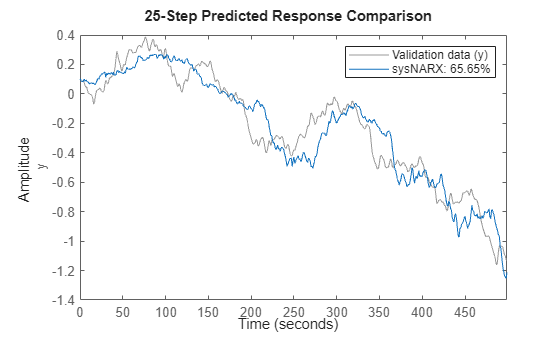
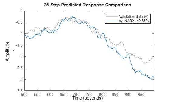
sysNARX provides an initial guess of the model coefficients. Check the model performance by computing 25-step-ahead forecasts.

Compare the 25-step-ahead prediction response of the model to the measured output in the training data set.

compare(TrainData,sysNARX,25)

Figure contains an axes object. The axes object with ylabel y contains 2 objects of type line. These objects represent Validation data (y), sysNARX: 65.65%.

Check the model performance on validation data.

compare(ValidateData,sysNARX,25)

Figure contains an axes object. The axes object with ylabel y contains 2 objects of type line. These objects represent Validation data (y), sysNARX: 42.65%.

Moving Average Model of the Residuals

Compute the prediction errors for the model, sysNARX, using the pe function.

errData = pe(TrainData,sysNARX,1);
stackedplot(errData)

Fit a linear moving average model to the signal in the timetable, errData. Assume a second order process.

nc = 2;
errMA = armax(errData,[0 nc])

errMA =
Discrete-time MA model: y(t) = C(z)e(t)
  C(z) = 1 + 0.6441 z^-1 + 0.1977 z^-2 
                                       
Sample time: 1 seconds
  
Parameterization:
   Polynomial orders:   nc=2
   Number of free coefficients: 2
   Use "polydata", "getpvec", "getcov" for parameters and their uncertainties.

Status:                                             
Estimated using ARMAX on time domain data "errData".
Fit to estimation data: 16.04% (prediction focus)   
FPE: 0.0003317, MSE: 0.0003291                      
 
Model Properties

Plot the residue correlation using resid.

resid(errData,errMA)

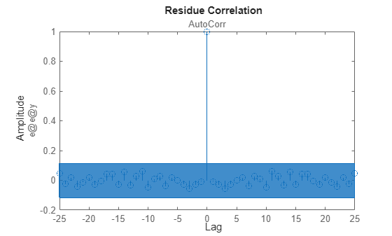
Figure contains an axes object. The axes object with title AutoCorr, ylabel e@e@y contains 2 objects of type line. One or more of the lines displays its values using only markers This object represents errMA.

The residual plot shows that the model, errMA, captures the essential dynamics embedded in the data, errData, because the residuals of this model are mostly uncorrelated at nonzero lags. The blue patch marks the region of statistical insignificance. At this point, an initial guess of the moving average term is the C(q) value for the NARMAX model.

errMA.C

ans = 1×3

    1.0000    0.6441    0.1977

Grey-Box Refinement of Model Parameters

The NARMAX model is a combination of the NARX model and a linear moving average term. Refine the initial estimates provided by sysNARX and errMA using a grey-box modeling approach. To speed up the refinement, this example fixes the parameters of sysNARX.

type('NARMAX_ODE.m') % ODE file

%------------------------------------------------------------------
function [dx, y] = NARMAX_ODE(~,x,u,fcn_par,C,varargin) 
%NARMAX_ODE ODE function for refining the coefficients of a NARMAX model 
% using a grey-box approach.
%
% The NARMAX model uses an additive moving average term.

% Copyright 2024 The MathWorks, Inc.

% If there are 2 moving average terms, the states are: 
% x1 := y(t-1)
% x2 := y(t-2)
% x3 := y_measured(t-1)
% x4 := y_measured(t-2)
% x5 := u(t-1)
% x6 := u(t-2)
% x7 := u(t-3)

% fcn_par -> coefficients used in f(.)
% C -> free coefficients of the moving average polynomial C(q)
% sys -> Nonlinear ARX model representing the function f(.)

% Separate out the parameters of the nonlinear sigmoidal function 
% and those corresponding to the moving average term
sys = varargin{1}{1};
nc = varargin{1}{2};
% sys = setpvec(sys, fcn_par); % not needed if fcn_par is fixed in the example
NL = sys.OutputFcn;
regressor_vector = x([nc+(1:2), end-2:end])';
y_NL = evaluate(NL,regressor_vector);
y_MA = C'*(x(nc+(1:nc))-x(1:nc));
y = y_NL + y_MA;
 
dx1 = y;
for k=1:nc-1
   dx1 = [dx1; x(k)]; %#ok<*AGROW>
end
dx1(end+1) = u(1);
for k=nc+(1:nc-1)
   dx1 = [dx1; x(k)];
end
dx2 = [u(2); x(end-2); x(end-1)];
dx = [dx1;dx2];

end
%------------------------------------------------------------------

Create the grey-box model using idnlgrey.

par1 = getpvec(sysNARX);
par2 = errMA.C(2:end)';
par = {par1,par2};
Orders = [1 2 7];
sysGrey_ini = idnlgrey("NARMAX_ODE",Orders,par,zeros(Orders(3),1),1,FileArgument={sysNARX, nc});
sysGrey_ini.Parameters(1).Fixed = 1; % Only update the MA coefficients.

Specify training options.

greyOpt = nlgreyestOptions(Display="on",SearchMethod="lsq");
Data_grey = iddata(TrainData.y,[TrainData.y TrainData.u],1,OutputName="y",InputName=["y","u"]);

Train the model using nlgreyest.

sysGrey = nlgreyest(Data_grey,sysGrey_ini,greyOpt)

sysGrey =

Discrete-time nonlinear grey-box model defined by 'NARMAX_ODE' (MATLAB file):

   x(t+Ts) = F(t, x(t), u(t), p1, p2, FileArgument)
      y(t) = H(t, x(t), u(t), p1, p2, FileArgument) + e(t)

 with 2 input(s), 7 state(s), 1 output(s), and 2 free parameter(s) (out of 74).

Sample time: 1 seconds

Status:                                                                                      
Estimated using Solver: FixedStepDiscrete; Search: lsqnonlin on time domain data "Data_grey".
Fit to estimation data: 94.96%                                                               
FPE: 0.0003595, MSE: 0.0003566                                                               

Model Properties

sysGrey is a one-step-ahead predictor of $y (k)$ .

You can use this model for multi-step-ahead prediction. The predictNARMAX.m function, which is attached to this example, performs multi-step-ahead predictions, including pure simulations. For multi-step-ahead predictions:

You can view an N-step-ahead prediction as a sequence of N one-step-ahead predictions.
In many engineering applications, a good model is one that can be used for simulation. Simulation is equivalent to an infinite-step-ahead prediction.

Next, use the trained model, sysGrey, to forecast the values of $y (k)$ . Computing just one-step-ahead prediction requires a simulation of the trained model.

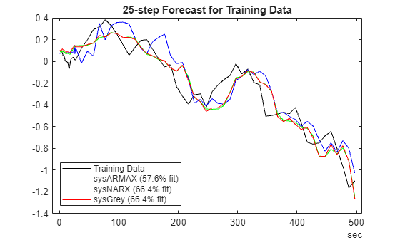
Set the prediction horizon to 25 samples, that is, predict the value of $y (k + 25)$ given data $y (i), u (i), i = 1, \dots, k$ . To save time, compute the forecasts for every 10th sample (see the variable SKIP in predictNARMAX.m).

H = 25;
plotPredictions(H,TrainData,sysARMAX,sysNARX,sysGrey);

Prediction started ...done.

Figure contains an axes object. The axes object with title 25-step Forecast for Training Data contains 4 objects of type line. These objects represent Training Data, sysARMAX (57.6% fit), sysNARX (66.4% fit), sysGrey (66.4% fit).

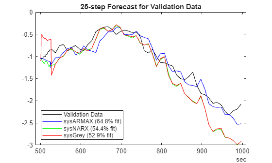
Similarly, generate the forecasting results for the validation data set.

plotPredictions(H,ValidateData,sysARMAX,sysNARX,sysGrey);

Prediction started ...done.

Figure contains an axes object. The axes object with title 25-step Forecast for Validation Data contains 4 objects of type line. These objects represent Validation Data, sysARMAX (64.8% fit), sysNARX (54.4% fit), sysGrey (52.9% fit).

Generic NARMAX Models

To directly model a time series as a NARMAX process with no additional simplifying assumptions regarding the nature of the contribution of the disturbances:

Create an extended model structure that uses two input sets: one corresponding to the measured outputs and the second corresponding to the measured exogenous inputs. Suppose the measured outputs are called $y_{m e a s}$ and the measured exogenous inputs are called $u$ . Then, the inputs of the extended model are $(y_{m e a s} (k), u (k))$ , while its output is the (one-step-ahead) predicted response, $y_{}^{\sim} (k)$ .
Prepare training data that uses samples of $y_{m e a s}$ as output and samples of $(y_{m e a s}, u)$ as inputs. In this training data set, $y_{m e a s}$ is being used as both the output time series and the exogenous input.
Train any suitable model structure for which the training algorithm is capable of minimizing simulation errors. Suitable model structures are nonlinear ARX models (with Focus="simulation"), nonlinear state-space models, nonlinear grey-box models, and Hammerstein-Wiener models. For the latter three structures, the training focus is always "simulation".
Use a specialized multi-step-ahead prediction method (such as predictNARMAX.m) to use the model to forecast outcomes.

Using Nonlinear ARX Models

Nonlinear ARX models are meant for autoregressive processes with no moving average terms, that is, NARX models but not NARMAX models. However, using the measured output $y (k)$ explicitly as an input allows you to use NARX models for identifying NARMAX models, as long as the training takes place in closed-loop (recurrent configuration). To use the measured output as the input, set the Focus option to "simulation" during model training.

Train the model for both one-step-ahead and infinite-horizon predictions. First, identify a one-step-ahead predictor model.

One-Step-Ahead Predictor Model

Create the regressors.

Reg = linearRegressor(["yp","y","u"],{1:2, 1:2, 1:3});  
getreg(Reg)

ans = 7×1 string
    "yp(t-1)"
    "yp(t-2)"
    "y(t-1)"
    "y(t-2)"
    "u(t-1)"
    "u(t-2)"
    "u(t-3)"

Create a nonlinear sigmoid function with two hidden layers of size five each using idNeuralNetwork.

NL = idNeuralNetwork([5 5],"sigmoid",NetworkType="RegressionNeuralNetwork");

Prepare training data that uses the measured outputs as additional input signals.

MultiInputTrainData = iddata(TrainData.y,[TrainData.y TrainData.u],1,...
   'OutputName',"yp",...
   'InputName',["y","u"]);

Prepare estimation options using nlarxOptions.

opt = nlarxOptions(Focus="simulation",Display="on",SearchMethod="lsq");
opt.Normalize = false;
opt.SearchOptions.MaxIterations = 100;

Train the model using nlarx.

sysNARMAXp = idnlarx("yp",["y","u"],Reg,NL);
sysNARMAXp.RegressorUsage{1:3,2} = false;
sysNARMAXp = nlarx(MultiInputTrainData,sysNARMAXp,opt)

sysNARMAXp =

Nonlinear ARX model with 1 output and 2 inputs
  Inputs: y, u
  Outputs: yp

Regressors:
  Linear regressors in variables yp, y, u
  List of all regressors

Output function: Regression neural network
Sample time: 1 seconds

Status:                                                         
Estimated using NLARX on time domain data "MultiInputTrainData".
Fit to estimation data: 95.47% (simulation focus)               
FPE: 0.0002511, MSE: 0.0002885                                  

Model Properties

Now, identify an infinite-step-ahead predictor model.

Infinite-Step-Ahead Predictor (Simulator) Model

Reg = linearRegressor(["y","u"],{1:2, 1:3});  
NL = idNeuralNetwork([5 5],"sigmoid",NetworkType="RegressionNeuralNetwork");
sysNARMAXs = nlarx(TrainData,Reg,NL,opt,OutputName="y")

sysNARMAXs =

Nonlinear ARX model with 1 output and 1 input
  Inputs: u
  Outputs: y

Regressors:
  Linear regressors in variables y, u
  List of all regressors

Output function: Regression neural network
Sample time: 1 seconds

Status:                                               
Estimated using NLARX on time domain data "TrainData".
Fit to estimation data: 62.53% (simulation focus)     
FPE: 0.0003108, MSE: 0.01971                          

Model Properties

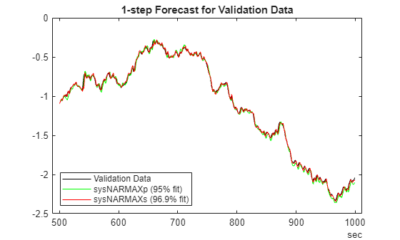
Assess the predictive abilities of these models for one-step-ahead prediction.

H = 1;

Generate forecasting results for the training data set.

plotPredictions(H,TrainData,sysNARMAXp,sysNARMAXs);

Prediction started ...done.

Figure contains an axes object. The axes object with title 1-step Forecast for Training Data contains 3 objects of type line. These objects represent Training Data, sysNARMAXp (95.5% fit), sysNARMAXs (95.9% fit).

Generate forecasting results for the validation data set.

plotPredictions(H,ValidateData,sysNARMAXp,sysNARMAXs);

Prediction started ...done.

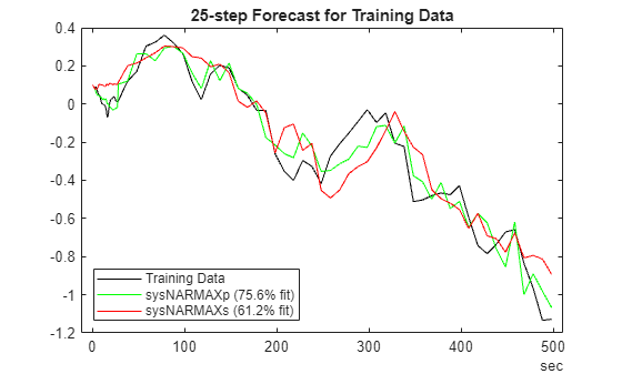
Figure contains an axes object. The axes object with title 1-step Forecast for Validation Data contains 3 objects of type line. These objects represent Validation Data, sysNARMAXp (95% fit), sysNARMAXs (96.9% fit).

Next, assess the predictive abilities of these models for 25-step-ahead prediction.

H = 25;

Generate forecasting results for the training data set.

plotPredictions(H,TrainData,sysNARMAXp,sysNARMAXs);

Prediction started ...done.

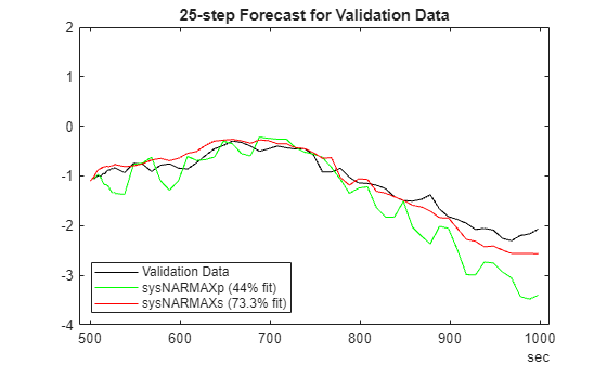
Figure contains an axes object. The axes object with title 25-step Forecast for Training Data contains 3 objects of type line. These objects represent Training Data, sysNARMAXp (75.6% fit), sysNARMAXs (61.2% fit).

Generate forecasting results for the validation data set.

plotPredictions(H,ValidateData,sysNARMAXp,sysNARMAXs);

Prediction started ...done.

ylim([-4 2])

Figure contains an axes object. The axes object with title 25-step Forecast for Validation Data contains 3 objects of type line. These objects represent Validation Data, sysNARMAXp (44% fit), sysNARMAXs (73.3% fit).

Using Neural State-Space Models

Now, create a predictive NARMAX model using neural state-space models. These models use deep networks from Deep Learning Toolbox™ to define the state-transition and output functions of a nonlinear state-space model.

Define the model states as:

$X (k) : = (y_{}^{\sim} (k - 1), y_{}^{\sim} (k - 2), y (k - 1), y (k - 2), u (k - 1), u (k - 2), u (k - 3))^{T}$ . Use this state definition to generate the state data. Create the regressors.

Reg = linearRegressor(["yp","y","u"],{1:2, 1:2, 1:3}); 

X = getreg(Reg, MultiInputTrainData);
X = X{4:end,:}; % Omit rows affected by initial conditions.
U = MultiInputTrainData;
U = U(4:end).u;

SSTrainData = iddata(X,U,1);
nx = 7; % 7 states
nu = 2; % 2 inputs

Create a discrete-time neural state-space model that uses seven states and two inputs using idNeuralStateSpace.

neuralSS_predict = idNeuralStateSpace(nx,NumInputs=nu,Ts=1);

Create a state-transition network with two hidden layers of size 50 each and sigmoid activation function using createMLPNetwork.

net = createMLPNetwork(neuralSS_predict,"state",LayerSizes=[50 50],Activations="sigmoid");
neuralSS_predict.StateNetwork = net;

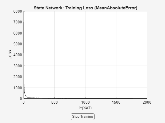
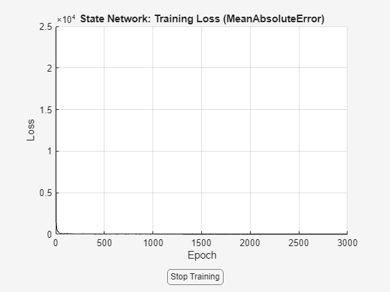
The nlssest command trains a neural state-space model. The training always aims at minimizing the simulation error, which is the goal of this example. For training the model:

Use ADAM as the training method.
Segment the data into overlapping segments of length 50 each. Use an overlap length of 10 samples.
Use a faster learning rate of 0.01. (The default rate is 0.001.)
Limit the number of training epochs to 2000.
Drop the learning rate by a factor of 0.1 every 700 epochs.

nnOpt = nssTrainingOptions("ADAM");
nnOpt.WindowSize = 50;
nnOpt.Overlap = 10;
nnOpt.MaxEpochs = 2000;
nnOpt.LearnRate = 0.01;
nnOpt.LearnRateSchedule='piecewise';
nnOpt.LearnRateDropPeriod = 700;

Train the model using the last data segment for in-training cross validation.

rng(1)
neuralSS_predict = nlssest(SSTrainData,neuralSS_predict,nnOpt,UseLastExperimentForValidation=true)

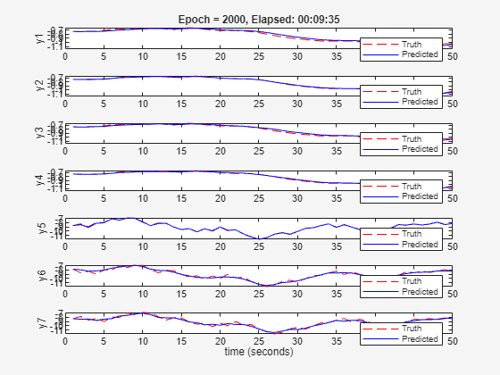
Figure Loss contains an axes object and another object of type uigridlayout. The axes object with title State Network: Training Loss (MeanAbsoluteError), xlabel Epoch, ylabel Loss contains an object of type animatedline.

Generating estimation report...done.

neuralSS_predict =

Discrete-time Neural ODE in 7 variables
     x(t+1) = f(x(t),u(t))
       y(t) = x(t) + e(t)
 
f(.) network:
  Deep network with 2 fully connected, hidden layers
  Activation function: sigmoid
 
Variables: x1, x2, x3, x4, x5, x6, x7
Sample time: 1 seconds
 
Status:                                                             
Estimated using NLSSEST on time domain data "SSTrainData".          
Fit to estimation data: [94.41;97.11;94.98;96.97;99.05;94.21;93.39]%
MSE: 0.2134                                                         

Model Properties

Similarly, you can directly train a response simulator. For training a simulator, you do not need to create an extended data set.

Reg = linearRegressor(["y","u"],{1:3, 1:3}); 
X = getreg(Reg,TT);
nx = width(X);
X = X{4:end,:}; % Omit rows affected by initial conditions.
U = TT.u(4:end);
AllData = iddata(X,U,1,OutputName=["y","x"+(2:nx)],InputName="u");
SSTrainData_sim = AllData(1:500);
SSValData_sim = AllData(501:end);

nu = 1; % only 1 input

Create a discrete-time neural state-space model that uses seven states and one input using the idNeuralStateSpace function.

neuralSS_sim = idNeuralStateSpace(nx,NumInputs=nu,Ts=1);

Create a state-transition network with two hidden layers of size 64 each and sigmoid activation function using the createMLPNetwork function.

net = createMLPNetwork(neuralSS_sim,"state",LayerSizes=[64 64],Activations="sigmoid");
neuralSS_sim.StateNetwork = net;
nnOpt.LearnRateDropPeriod = 1000;
nnOpt.MaxEpochs = 3000;
nnOpt.LearnRate = 0.1;

Train the model.

rng(1)
neuralSS_sim = nlssest(SSTrainData_sim, neuralSS_sim, nnOpt, UseLastExperimentForValidation=true)

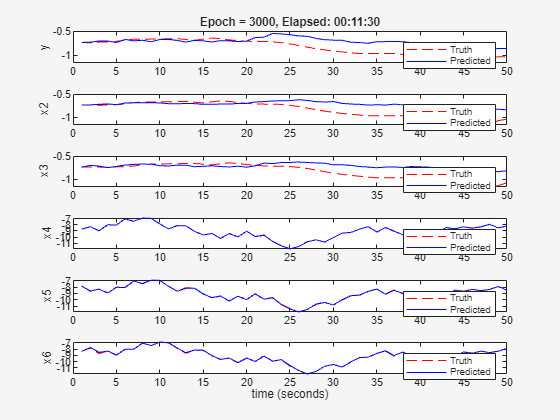
Generating estimation report...done.

neuralSS_sim =

Discrete-time Neural ODE in 6 variables
     x(t+1) = f(x(t),u(t))
       y(t) = x(t) + e(t)
 
f(.) network:
  Deep network with 2 fully connected, hidden layers
  Activation function: sigmoid
 
Variables: x1, x2, x3, x4, x5, x6
Sample time: 1 seconds
 
Status:                                                       
Estimated using NLSSEST on time domain data "SSTrainData_sim".
Fit to estimation data: [74.7;76.09;76.28;99.56;99.31;99.05]% 
MSE: 0.02943                                                  

Model Properties

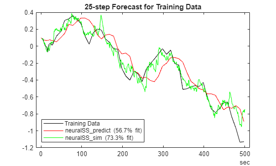
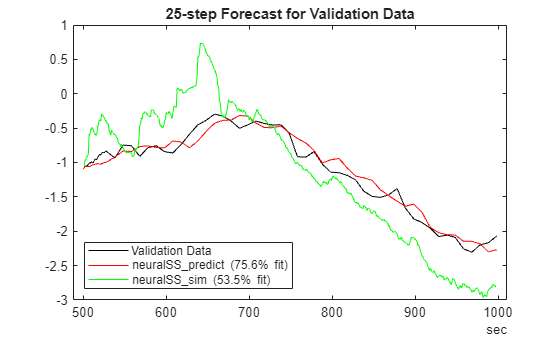
Use the model to predict 25 steps into the future for both the training and validation data sets.

H = 25;
plotPredictions(H,TrainData,neuralSS_predict);

Prediction started ...done.

hold on
yp = predict(neuralSS_sim,SSTrainData_sim,H); 
yp=yp.y;
FitPercent = (1-goodnessOfFit(SSTrainData_sim.y(:,1),yp(:,1),'nrmse'))*100

FitPercent = 
73.3235

p = plot(SSTrainData_sim.SamplingInstants,yp(:,1),'g');
p.DisplayName = sprintf('neuralSS\\_sim (%2.3g%% fit)',FitPercent);
hold off

$Figure contains an axes object. The axes object with title 25-step Forecast for Training Data contains 3 objects of type line. These objects represent Training Data, neuralSS\_predict (56.7% fit), neuralSS\_sim (73.3% fit).$

plotPredictions(H,ValidateData,neuralSS_predict);

Prediction started ...done.

hold on
ypv = predict(neuralSS_sim,SSValData_sim,H); 
ypv=ypv.y;
FitPercent = (1-goodnessOfFit(SSValData_sim.y(:,1),ypv(:,1),'nrmse'))*100

FitPercent = 
53.4840

p = plot(SSValData_sim.SamplingInstants,ypv(:,1),'g');
p.DisplayName = sprintf('neuralSS\\_sim (%2.3g%% fit)',FitPercent);
hold off

$Figure contains an axes object. The axes object with title 25-step Forecast for Validation Data contains 3 objects of type line. These objects represent Validation Data, neuralSS\_predict (75.6% fit), neuralSS\_sim (53.5% fit).$

Going from a NARX to a NARMAX model means that the one-step-ahead response predictor becomes recursive (see predictNARMAX.m) and hence takes longer to compute the results. But the benefit is that the one-step-ahead predictions are more accurate for systems whose output measurement depends on both the present and the past disturbances.

Alternatively, directly train a nonlinear model for simulation fidelity (see the models sysNARMAXs and neuralSS_sim in this example). You can use such a model for finite-horizon prediction too, although it will have no mechanism for correcting the predictions based on most recent output measurements.

Simulation Capability

Finally, compare the simulation ability of the trained models (that is, forecast infinitely into the future). Set the prediction horizon to Inf. This setting means you are practically forecasting to the length of the available data. For validation data, this setting implies a horizon of 500.

H = Inf;
plotPredictions(H, ValidateData, ...
   sysARMAX, ... linear ARMAX model
   sysNARX, ... nonlinear ARX model (no MA term)
   sysNARMAXp, ... nonlinear ARMAX model trained to minimize one-step prediction error
   sysNARMAXs, ...nonlinear ARMAX model trained to minimize simulation error
   sysGrey, ... nonlinear ARX model and additive linear MA model
   neuralSS_predict ... neural state-space model trained to minimize one-step prediction error
   );

Prediction started ...done.
Prediction started ...done.
Prediction started ...done.

ylim([-4 2])

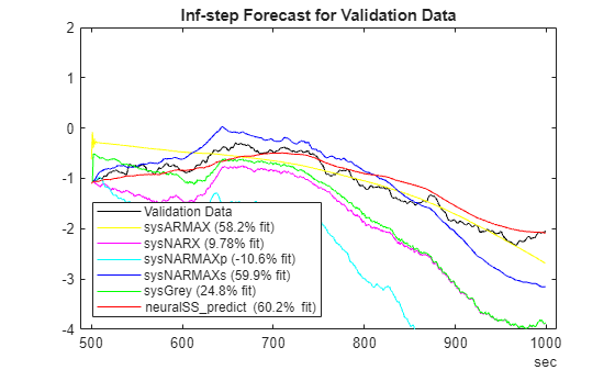
$Figure contains an axes object. The axes object with title Inf-step Forecast for Validation Data contains 7 objects of type line. These objects represent Validation Data, sysARMAX (58.2% fit), sysNARX (9.78% fit), sysNARMAXp (-10.6% fit), sysNARMAXs (59.9% fit), sysGrey (24.8% fit), neuralSS\_predict (60.2% fit).$

As shown by the fit percentages, forecasting indefinitely into the future is a demanding goal for models of NARMAX processes.