NARMAX Model Identification

This topic describes some ways to identify nonlinear autoregressive moving average with exogenous inputs (NARMAX) models. These models are currently not available in the System Identification Toolbox™ software. However, this topic shows how to identify NARMAX models using the available model structures and their training algorithms by preparing a finite-horizon prediction algorithm.

Linear Autoregressive Models

NARMAX models are nonlinear counterparts of the linear autoregressive models that are popular structures used to forecast the outcomes of time series. To understand the structure of a NARMAX model, it is helpful to review the simpler, linear versions first.

AR Models

The simplest form of a linear autoregressive model (AR) is

$y (k) + a_{1} y (k - 1) + a_{2} y (k - 2) + \dots = e (k)$

$A (q) y (k) = e (k),$

where $A (q) : = 1 + a_{1} q^{- 1} + a_{2} q^{- 2} + \dots$ is a polynomial in the shift operator q^-1, that is, q^-iy(k) = y(k-i).

The expression y(k) describes the time series under observation and e(k) is the disturbance process. Thus, y(k) is generated by a weighted sum of its own past values but is corrupted by the noise, e(k). This is called the data-generating system, also known as the true system. In engineering applications, y(k) is typically obtained by sampling a signal of physical origin, y(t), such as vibrations measured using an accelerometer. When y(t) is sampled uniformly using a sampling interval (sample time) of T_s, it leads to the measurements y(T_s),y(2T_s),...,y(NT_s), where k = 1,...,N are the sampling instants. Typically, e(t) is assumed to be a zero-mean independent and identically distributed Gaussian process. Then, given the measurements y(k), k = 1,2,...,T, the prediction of the response at the next time instant, T + 1, is given by

$\tilde{y} (T + 1) = - a_{1} y (T) - a_{2} y (T - 1) + \dots .$

This equation is called the one-step-ahead predictor for the process y(k). The equation predicts the value of y exactly one step into the future.

ARX Models

When exogenous but measurable influences, u(k), affect y(k), the data-generating system equation is

$y (k) + a_{1} y (k - 1) + a_{2} y (k - 2) + \dots = b_{0} u (k) + b_{1} u (k - 1) + \dots + e (k),$

or more succinctly

$A (q) y (k) = B (q) u (k) + e (k),$

where $A (q) : = 1 + a_{1} q^{- 1} + a_{2} q^{- 2} + \dots$ and $B (q) : = b_{0} + b_{1} q^{- 1} + \dots .$

This model is called an autoregressive with exogenous inputs (ARX) model. Some observations regarding the ARX model structure are:

u(k) is supposed to be known or measured with no noise. That is, practically, any measurement errors in u(k) are combined into the fictitious noise source e(k).
The model regressors are the lagged variables y(k-1),y(k-2),...,u(k),u(k-1),u(k-2),.... At time instant k, the regressors are fully known.
In engineering applications, y(t) is referred to as an output signal and u(t) as an input signal. Thus, the data-generating system equation is an input-output model.

The one-step-ahead predictor takes the form

$\tilde{y} (k + 1) = - a_{1} y (k) - a_{2} y (k - 1) + \dots + b_{0} u (k + 1) + b_{1} u (k) + b_{2} u (k - 1) + \dots .$

You can also express an ARX model in the state-space form by defining the states using the lagged variables.

ARMA Models

The predictor of the AR or ARX model is a static equation, that is, the terms on the right-hand side of the predictor equations are fully known at the time instant k without needing to look up their past values. However, when the output in the data-generating system is affected by not just the current value of the disturbance e(k) but also its past values (e(k-1),e(k-2), and so on), the equation gets more complicated. For example, the form of an autoregressive with moving average (ARMA) model is

$y (k) = a_{1} y (k - 1) + a_{2} y (k - 2) + \dots + e (k) + c_{1} e (k - 1) + c_{2} e (k - 2) + \dots .$

Here, the one-step-ahead prediction of y(k) is not as straightforward as in the ARX model. To estimate ỹ(k + 1), you need to know the past predictions (ỹ(k),ỹ(k-1),...).

An ARMA predictor takes the form

$\tilde{y} (k) = a_{1} y (k - 1) + a_{2} y (k - 2) + \dots + c_{1} (y (k - 1) - \tilde{y} (k - 1)) + c_{2} (y (k - 2) - \tilde{y} (k - 2)) + \dots,$

which can be rearranged to

$\tilde{y} (k) + c_{1} \tilde{y} (k - 1) + \tilde{y} (k - 2) + \dots = (a_{1} + c_{1}) y (k - 1) + (a_{2} + c_{2}) y (k - 2) + ....$

This equation is an autoregressive equation. That is, you do not know the value of ỹ(k) in advance. Only the initial value or initial guess for ỹ(1) is available. You must simulate this model by using the initial guess ỹ(1) to solve for ỹ(2), and then use the values ỹ(1),ỹ(2) to solve for ỹ(3), and so on.

ARMAX Models

When exogenous inputs are present, the ARMA model becomes an ARMAX model. The form of an ARMAX model is

$y (k) = a_{1} y (k - 1) + a_{2} y (k - 2) + \dots + b_{0} u (k) + b_{1} u (k - 1) + \dots + e (k) + c_{1} e (k - 1) + c_{2} e (k - 2) + \dots .$

Nonlinear Autoregressive Models

From the predictor for the ARX model, note that:

The regressors are all lagged versions of the measured variables y(k) and u(k) with no other transformations.
The prediction uses a weighted sum of the regressors.

NARX Models

For a nonlinear extension of the linear ARX predictor:

In place of linear regressors (y(k - 1),y(k - 2),...,u(k - 1),...), you can use nonlinear transformations such as polynomials or trigonometric transformations of the lagged variables, for example, y(k - 1)², y(k - 4)u(k - 6), sin(3u(t - 5)), |u(t)|³,..., and so on.
You can replace the simple weighted sum with a more complicated nonlinear map such as sigmoids or wavelets.

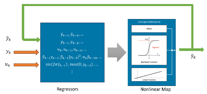
Nonlinear ARX (NARX) models facilitate such extensions. The general form of these models is

$y (k) = f (r_{1} (k), r_{2} (k), ...) + e (k),$

where r₁(k),r₂(k),... are the model regressors. For example, r₁(k) = y(k-1), r₂(k) = y(k-5)², r₃(k) = sin(2πu(k)), and so on. A simpler notation for the NARX models is

$y (k) = f (y (k - 1), y (k - 2), \dots, u (k), u (k - 1), \dots) + e (k),$

where it is understood that the lagged variables can undergo additional transformations (polynomial, trigonometric, and so on) before being passed as input arguments to the mapping function, $f (\cdot)$ .

You represent the NARX models with idnlarx objects and train them using the nlarx command.

NARMAX Models

Similar to the linear case, you can extend the NARX model to allow for dependence on the past prediction errors leading to the NARMAX model form

$y (k) = f (y (k - 1), y (k - 2), \dots, u (k), u (k - 1), \dots, e (k - 1), e (k - 2), \dots) + e (k) .$

In this form, you can view e(k - 1),e(k - 2),... as extra regressors whose values are not known directly. At time k, e(k - i) = y(t - i) - ỹ(t - i), so the form of the one-step-ahead predictor is

$\tilde{y} (k + 1) = f (y (k), y (k - 1), \dots, u (k + 1), u (k), u (k - 1), \dots, \tilde{y} (k), \tilde{y} (k - 1), \tilde{y} (k - 2), \dots) .$

Because the predictions depend on their own past values, to determine ỹ(k + 1), you must simulate the model. Start at ỹ(1) and march forward to the current time instant k. This simulation makes the prediction more time-consuming. Also, determining $f (\cdot)$ by model training is more complex due to the recursive nature of the prediction.

NARMAX Models with Linear and Additive Moving Average Term. Consider the data-generating system

$y (k) = f (y (k - 1), y (k - 2), \dots, u (k), u (k - 1), \dots) + C (q) e (k) .$

Here, the contribution of the error terms is written as a separate additive term C(q)e(k) = e(k) + c₁e(k - 1) + c₂e(k - 2) + .... The one-step-ahead predictor is

$\tilde{y} (k + 1) = f (y (k), y (k - 1), \dots, u (k + 1), u (k), u (k - 1), \dots) + c_{1} (y (k) - \tilde{y} (k)) + c_{2} (y (k - 1) - \tilde{y} (k - 1)) + \dots,$

You can rearrange the predicted quantities to

$C (q) \tilde{y} (k + 1) = f (y (k), y (k - 1), \dots, u (k + 1), u (k), u (k - 1), \dots) + c_{1} y (k) + c_{2} y (k - 1) + \dots,$

where C(q) = 1 + c₁q^-1 + c₂q^-2 + .... This equation represents an autoregressive model for the process ỹ(k + 1). This equation is driven by the inputs y(k) and u(k) which are assumed to be known at time instant k. For training this model using input and output measurements, {u(k), y(k)}, k = 1,2,...,N, you need to determine the values of the coefficients (such as weights and biases) used by the nonlinear function, $f (\cdot)$ , and the coefficients c₁,c₂,... used by the moving average terms.

Generic NARMAX Models. In general, you do not know the nature of the dependence of the output y(k) on the error terms e(k - 1),e(k - 2),.... Using e(k) = y(k) - ỹ(k), a generic form of the NARMAX predictor is:

$\tilde{y} (k) = f (\tilde{y} (k - 1), \tilde{y} (k - 2), \dots y (k - 1), y (k - 2), \dots, u (k), u (k - 1), \dots) .$

This model uses the measured processes y(k) and u(k) as inputs and generates ỹ(k) as the response. So you can approximate the function, $f (\cdot)$ , using a black-box model. You can use neural networks as generic forms of the function using either nonlinear ARX models or neural state-space models.

For a detailed example that shows how to generate NARMAX models using these model structures, see Generate NARMAX Models.