Continuous-Discrete Conversion Methods

System Identification Toolbox™ offers several discretization and interpolation methods for converting identified dynamic system models between continuous time and discrete time and for resampling discrete-time models. Some methods tend to provide a better frequency-domain match between the original and converted systems, while others provide a better match in the time domain. Use the following table to help select the method that is best for your application.

Discretization Method	Use When
Zero-Order Hold	You want an exact discretization in the time domain for staircase inputs.
First-Order Hold	You want an exact discretization in the time domain for piecewise linear inputs.
Impulse-Invariant Mapping (continuous-to-discrete conversion only)	You want an exact discretization in the time domain for impulse train inputs.
Tustin Approximation	You want good matching in the frequency domain between the continuous- and discrete-time models. Your model has important dynamics at some particular frequency.
Zero-Pole Matching Equivalents	You have a SISO model. You want good matching in the frequency domain between the continuous- and discrete-time models.
Least Squares (Control System Toolbox) (continuous-to-discrete conversion only)	You have a SISO model. You want good matching in the frequency domain between the continuous- and discrete-time models. You want to capture fast system dynamics but must use a larger sample time.

For information about how to specify a conversion method at the command line, see c2d, d2c, and d2d. You can experiment interactively with different discretization methods in the Live Editor using the Convert Model Rate (Control System Toolbox) task (requires a license).

Zero-Order Hold

The Zero-Order Hold (ZOH) method provides an exact match between the continuous- and discrete-time systems in the time domain for staircase inputs.

The following block diagram illustrates the zero-order-hold discretization H_d(z) of a continuous-time linear model H(s).

The ZOH block generates the continuous-time input signal u(t) by holding each sample value u(k) constant over one sample period:

$$u\left(t\right)=u\left[k\right],k{T}_s\le t\le \left(k+1\right)T_s$$

The signal u(t) is the input to the continuous system H(s). The output y[k] results from sampling y(t) every T_s seconds.

Conversely, given a discrete system H_d(z), d2c produces a continuous system H(s). The ZOH discretization of H(s) coincides with H_d(z).

The ZOH discrete-to-continuous conversion has the following limitations:

• d2c cannot convert LTI models with poles at z = 0.

• For discrete-time LTI models having negative real poles, ZOH d2c conversion produces a continuous system with higher order. The model order increases because a negative real pole in the z domain maps to a pure imaginary value in the s domain. Such mapping results in a continuous-time model with complex data. To avoid this issue, the software instead introduces a conjugate pair of complex poles in the s domain.

ZOH Method for Systems with Time Delays

You can use the ZOH method to discretize SISO or MIMO continuous-time models with time delays. The ZOH method yields an exact discretization for systems with input delays, output delays, or transport delays.

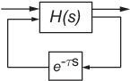
For systems with internal delays (delays in feedback loops), the ZOH method results in approximate discretizations. The following figure illustrates a system with an internal delay.

For such systems, c2d performs the following actions to compute an approximate ZOH discretization:

1. Decomposes the delay τ as $$\tau =k{T}_s+\rho$$ with $$0\le \rho <T_s$$.

2. Absorbs the fractional delay $$\rho$$ into H(s).

3. Discretizes H(s) to H(z).

4. Represents the integer portion of the delay kT_s as an internal discrete-time delay z^–k. The final discretized model appears in the following figure:

First-Order Hold

The First-Order Hold (FOH) method provides an exact match between the continuous- and discrete-time systems in the time domain for piecewise linear inputs.

FOH differs from ZOH by the underlying hold mechanism. To turn the input samples u[k] into a continuous input u(t), FOH uses linear interpolation between samples:

$$u\left(t\right)=u\left[k\right]+\frac{t-k{T}_s}{T_s}\left(u\left[k+1\right]-u\left[k\right]\right),k{T}_s\le t\le \left(k+1\right)T_s$$

In general, this method is more accurate than ZOH for systems driven by smooth inputs.

This FOH method differs from standard causal FOH and is more appropriately called triangle approximation (see [2], p. 228). The method is also known as ramp-invariant approximation.

FOH Method for Systems with Time Delays

You can use the FOH method to discretize SISO or MIMO continuous-time models with time delays. The FOH method handles time delays in the same way as the ZOH method. See ZOH Method for Systems with Time Delays.

Impulse-Invariant Mapping

The impulse-invariant mapping produces a discrete-time model with the same impulse response as the continuous time system. For example, compare the impulse response of a first-order continuous system with the impulse-invariant discretization:

G = tf(1,[1,1]);
Gd1 = c2d(G,0.01,'impulse');
impulse(G,Gd1)

The impulse response plot shows that the impulse responses of the continuous and discretized systems match.

Impulse-Invariant Mapping for Systems with Time Delays

You can use impulse-invariant mapping to discretize SISO or MIMO continuous-time models with time delays, except that the method does not support ss models with internal delays. For supported models, impulse-invariant mapping yields an exact discretization of the time delay.

Tustin Approximation

The Tustin or bilinear approximation yields the best frequency-domain match between the continuous-time and discretized systems. This method relates the s-domain and z-domain transfer functions using the approximation:

$$z=e^{s{T}_s}\approx \frac{1+s{T}_s/2}{1-s{T}_s/2}.$$

In c2d conversions, the discretization H_d(z) of a continuous transfer function H(s) is:

$$H_d\left(z\right)=H\left(s^{\prime }\right),s^{\prime }=\frac{2}{T_s}\frac{z-1}{z+1}$$

Similarly, the d2c conversion relies on the inverse correspondence

$$H\left(s\right)=H_d\left(z^{\prime }\right),z^{\prime }=\frac{1+s{T}_s/2}{1-s{T}_s/2}$$

When you convert a state-space model using the Tustin method, the states are not preserved. The state transformation depends upon the state-space matrices and whether the system has time delays. For example, for an explicit (E = I) continuous-time model with no time delays, the state vector w[k] of the discretized model is related to the continuous-time state vector x(t) by:

$$w\left[k{T}_s\right]=\left(I-A\frac{T_s}{2}\right)x\left(k{T}_s\right)-\frac{T_s}{2}Bu\left(k{T}_s\right)=x\left(k{T}_s\right)-\frac{T_s}{2}\left(Ax\left(k{T}_s\right)+Bu\left(k{T}_s\right)\right).$$

T_s is the sample time of the discrete-time model. A and B are state-space matrices of the continuous-time model.

The Tustin approximation is not defined for systems with poles at z = –1 and is ill-conditioned for systems with poles near z = –1.

Tustin Approximation with Frequency Prewarping

If your system has important dynamics at a particular frequency that you want the transformation to preserve, you can use the Tustin method with frequency prewarping. This method ensures a match between the continuous- and discrete-time responses at the prewarp frequency.

The Tustin approximation with frequency prewarping uses the following transformation of variables:

$$H_d\left(z\right)=H\left(s^{\prime }\right),s^{\prime }=\frac{\omega }{\tan \left(\omega T_s/2\right)}\frac{z-1}{z+1}$$

This change of variable ensures the matching of the continuous- and discrete-time frequency responses at the prewarp frequency ω, because of the following correspondence:

$$H\left(j\omega \right)=H_d\left(e^{j\omega T_s}\right)$$

Tustin Approximation for Systems with Time Delays

You can use the Tustin approximation to discretize SISO or MIMO continuous-time models with time delays.

By default, the Tustin method rounds any time delay to the nearest multiple of the sample time. Therefore, for any time delay tau, the integer portion of the delay, k*Ts, maps to a delay of k sampling periods in the discretized model. This approach ignores the residual fractional delay, tau - k*Ts.

You can approximate the fractional portion of the delay by a discrete all-pass filter (Thiran filter) of specified order. To do so, use the ThiranOrder option of c2dOptions.

To understand how the Tustin method handles systems with time delays, consider the following SISO state-space model G(s). The model has input delay τ_i, output delay τ_o, and internal delay τ.

The following figure shows the general result of discretizing G(s) using the Tustin method.

By default, c2d converts the time delays to pure integer time delays. The c2d command computes the integer delays by rounding each time delay to the nearest multiple of the sample time T_s. Thus, in the default case, m_i = round(τ_i/T_s), m_o = round(τ_o/T_s), and m = round(τ/T_s).. Also in this case, F_i(z) = F_o(z) = F(z) = 1.

If you set ThiranOrder to a non-zero value, c2d approximates the fractional portion of the time delays by Thiran filters F_i(z), F_o(z), and F(z).

The Thiran filters add additional states to the model. The maximum number of additional states for each delay is ThiranOrder.

For example, for the input delay τ_i, the order of the Thiran filter F_i(z) is:

order(F_i(z)) = max(ceil(τ_i/T_s), ThiranOrder).

If ceil(τ_i/T_s) < ThiranOrder, the Thiran filter F_i(z) approximates the entire input delay τ_i. If ceil(τ_i/T_s) > ThiranOrder, the Thiran filter only approximates a portion of the input delay. In that case, c2d represents the remainder of the input delay as a chain of unit delays z^–m_i, where

m_i = ceil(τ_i/T_s) – ThiranOrder

c2d uses Thiran filters and ThiranOrder in a similar way to approximate the output delay τ_o and the internal delay τ.

When you discretizetf and zpk models using the Tustin method, c2d first aggregates all input, output, and transport delays into a single transport delay τ_TOT for each channel. c2d then approximates τ_TOT as a Thiran filter and a chain of unit delays in the same way as described for each of the time delays in ss models.

For more information about Thiran filters, see the thiran (Control System Toolbox) reference page and [4].

Zero-Pole Matching Equivalents

This method of conversion, which computes zero-pole matching equivalents, applies only to SISO systems. The continuous and discretized systems have matching DC gains. Their poles and zeros are related by the transformation:

$$z_i=e^{s_i{T}_s}$$

where:

• z_i is the ith pole or zero of the discrete-time system.

• s_i is the ith pole or zero of the continuous-time system.

• T_s is the sample time.

See [2] for more information.

Zero-Pole Matching for Systems with Time Delays

You can use zero-pole matching to discretize SISO continuous-time models with time delay, except that the method does not support ss models with internal delays. The zero-pole matching method handles time delays in the same way as the Tustin approximation. See Tustin Approximation for Systems with Time Delays.

Least Squares

The least squares method minimizes the error between the frequency responses of the continuous-time and discrete-time systems up to the Nyquist frequency using a vector-fitting optimization approach. This method is useful when you want to capture fast system dynamics but must use a larger sample time, for example, when computational resources are limited.

This method is supported only by the c2d function and only for SISO systems.

As with Tustin approximation and zero-pole matching, the least squares method provides a good match between the frequency responses of the original continuous-time system and the converted discrete-time system. However, when using the least squares method with:

• The same sample time as Tustin approximation or zero-pole matching, you get a smaller difference between the continuous-time and discrete-time frequency responses.

• A lower sample time than what you would use with Tustin approximation or zero-pole matching, you can still get a result that meets your requirements. Doing so is useful if computational resources are limited, since the slower sample time means that the processor must do less work.

References

[1] Åström, K.J. and B. Wittenmark, Computer-Controlled Systems: Theory and Design, Prentice-Hall, 1990, pp. 48-52.

[2] Franklin, G.F., Powell, D.J., and Workman, M.L., Digital Control of Dynamic Systems (3rd Edition), Prentice Hall, 1997.

[3] Smith, J.O. III, "Impulse Invariant Method", Physical Audio Signal Processing, August 2007. https://www.dsprelated.com/dspbooks/pasp/Impulse_Invariant_Method.html.

[4] T. Laakso, V. Valimaki, "Splitting the Unit Delay", IEEE Signal Processing Magazine, Vol. 13, No. 1, p.30-60, 1996.