Convert Model Rate
Convert models between continuous time and discrete time and resample models in the Live Editor
Description
Convert Model Rate lets you interactively convert an LTI model between continuous time and discrete time. You can also use it to resample a discrete-time model. The task automatically generates MATLAB® code for your live script.
To get started with the Convert Model Rate task, select the model you want to convert. You can also specify the target sample time, conversion method, and other parameters. The task generates the converted model in the MATLAB workspace, and can generate a response plot to let you monitor the match between the original and converted models as you experiment with conversion parameters.
Open the Task
To add the Convert Model Rate task to a live script in the MATLAB Editor:
On the Live Editor tab, select Task > Convert Model Rate.
In a code block in your script, type a relevant keyword, such as
convert,rate, orc2d. SelectConvert Model Ratefrom the suggested command completions.
Examples
Use the Convert Model Rate task in the Live Editor to interactively convert a model from continuous time to discrete time. Experiment with different methods, options, and response plots. The task automatically generates code reflecting your selections. Open this example to see a preconfigured script containing the Convert Model Rate task.
Create a continuous-time transfer-function model.
G = tf([1 -50 300],[1 3 200 350]);
To discretize this model, open the Convert Model Rate task in the Live Editor. On the Live Editor tab, select Task > Convert Model Rate. In the task, select G as the model to convert.
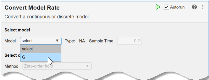
The task automatically discretizes the model using the default sample time, 0.2 s, and the default conversion method, Zero-order hold. It also creates a Bode plot, allowing you to compare the responses of the original and converted models.
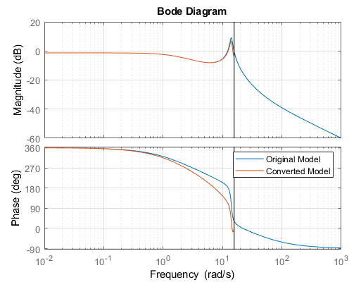
The vertical line on the plot shows the Nyquist frequency associated with the default sample time. Suppose you want to use a sample time of 0.15 seconds. Change the sample time by entering the new value in the Sample Time field. The response plot automatically updates to reflect the new sample time.
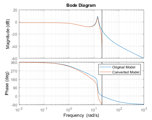
If the precise dynamics of the resonance are important for your application, you can improve the frequency-domain match using a different conversion method. In the task, try experimenting with different methods and observe their effect on the response plot.
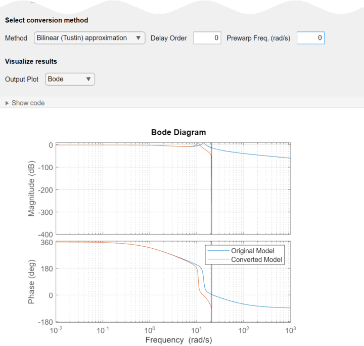
The Tustin method can yield a better match in the frequency domain than the default zero-order hold method. (See Continuous-Discrete Conversion Methods.) In Select Conversion Method, select Bilinear (Tustin) approximation. Initially, the resulting frequency-domain match is poorer than with the zero-order hold method.
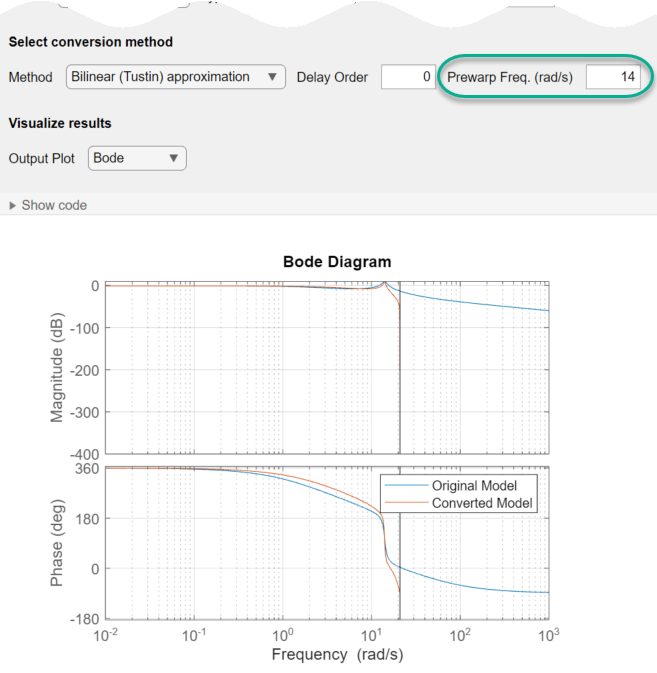
You can improve the match using a prewarp frequency. This option forces the discrete-time response to match at the frequency you specify. The resonance of G peaks at about 14 rad/s. Enter that value for the prewarp frequency. The match does improve around the resonance. However, the resonance is very close to the Nyquist frequency for the sample time of 0.15 s, which limits how close the match can be.
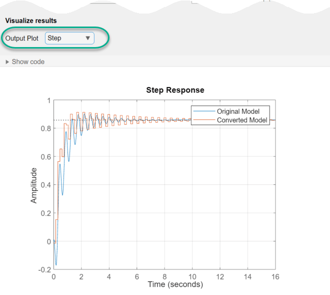
The Convert Model Rate task can generate other types of response plots. For instance, to compare the time-domain responses of the original and converted model, in Output Plot, select step or impulse.
The task generates code in your live script. The generated code reflects the parameters and options you select, and includes code to generate the response plot you specify. To see the generated code, click ![]() Show code at the bottom of the task parameter area. The task expands to display the generated code.
Show code at the bottom of the task parameter area. The task expands to display the generated code.
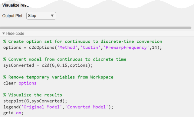
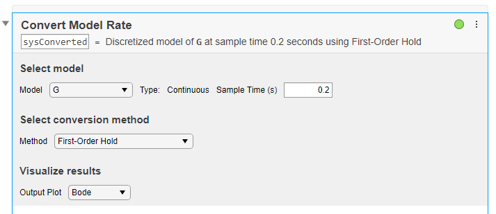
By default, the generated code uses sysConverted as the name of the output variable, which is the converted model. To specify a different output-variable name, enter the new name in the summary line at the top of the task. For instance, change the name to sys_d.
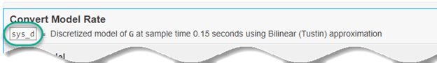
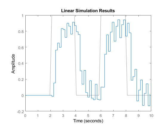
The task updates the generated code to reflect the new variable name, and the new converted model sys_d appears in the MATLAB workspace. You can use the model for further analysis or control design as you would any other model object. For instance, simulate the converted system's response to a square-wave input. Use the sample time you specified in the task.
[u,t] = gensig('square',4,10,0.15);
lsim(sys_d,u,t)
Parameters
Version History
Introduced in R2019b