Optimize Simulink Model in Parallel
This example shows how to optimize a Simulink® model in parallel using several Global Optimization Toolbox solvers. The example uses vectorized computations that internally call parsim to perform the parallel computations.
Model and Objective Function
The Lorenz system is a system of ordinary differential equations (see Lorenz system). For real constants , and the system is
Lorenz's values of the parameters for a sensitive system are and . Start the system from [x(0),y(0),z(0)] = [10,20,10] and view the evolution of the system from time 0 through 100.
sigma = 10;
beta = 8/3;
rho = 28;
f = @(t,a) [-sigma*a(1) + sigma*a(2); rho*a(1) - a(2) - a(1)*a(3); -beta*a(3) + a(1)*a(2)];
xt0 = [10,20,10];
[tspan,a] = ode45(f,[0 100],xt0);     % Runge-Kutta 4th/5th order ODE solver
figure
plot3(a(:,1),a(:,2),a(:,3))
view([-10.0 -2.0])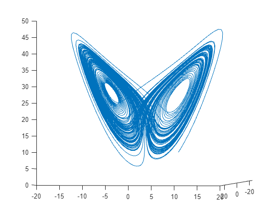
The evolution is quite complicated. But over a small time interval, the system looks somewhat like uniform circular motion. Plot the solution over the time interval [0,1/10].
[tspan,a] = ode45(f,[0 1/10],xt0);     % Runge-Kutta 4th/5th order ODE solver
figure
plot3(a(:,1),a(:,2),a(:,3))
view([-30 -70])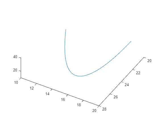
Uniform circular motion relies on several parameters:
Angle of the path from the x-y plane
Angle of the plane from a tilt along the x-axis
Speed
Radius
Time offset
3-D offset
For details relating these parameters to uniform circular motion and fitting them to a Lorenz system, see the example Fit an Ordinary Differential Equation (ODE).
The objective function is to minimize the sum of squares of the difference between the Lorenz system and the uniform circular motion over a set of times from 0 through 1/10. For times xdata, the objective function is
objective = sum((fitlorenzfn(x,xdata) - lorenz(xdata)).^2) - (F(1) + F(end))/2
Here, fitlorenzfn computes points on the uniform circular motion path, lorenz(xdata) represents the 3-D evolution of the Lorenz system at times xdata, and F represents the vector of squared distances between corresponding points in the circular and Lorenz systems. The objective subtracts half of the values at the endpoints to best approximate an integral.
Consider the uniform circular motion as the curve to match, and modify the Lorenz parameters in the simulation to minimize the objective function.
Simulink Model
The Lorenz_system.slx file, available when you run this example, implements the Lorenz system.
Enter the data for the uniform circular motion.
x = zeros(8,1);
x(1) = 1.2814;
x(2) = -1.4930;
x(3) = 24.9763;
x(4) = 14.1870;
x(5) = 0.0545;
x(6:8) = [13.8061;1.5475;25.3616];
Load the Lorenz system and simulate it with the base parameters. Create a 3-D plot of the resulting system and compare it with the uniform circular motion.
model = "Lorenz_system";
open_system(model);
in = Simulink.SimulationInput(model);
% params [X0,Y0,Z0,Sigma,Beta,Rho]
params = [10,20,10, 10,8/3,28]; % The original parameters Sigma, Beta, Rho
in = setparams(in,model,params);
out = sim(in);

yout = out.yout;
h = figure;
plot3(yout{1}.Values.Data,yout{2}.Values.Data,yout{3}.Values.Data,"gx");
view([-30 -70])

tlist = yout{1}.Values.Time;
YDATA = fitlorenzfn(x,tlist);
hold on
plot3(YDATA(:,1),YDATA(:,2),YDATA(:,3),"kx")
hold off
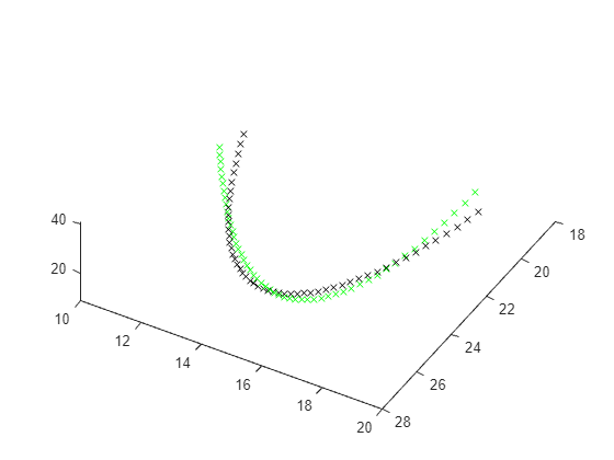
Calculate the sum of squares of the differences between the curves for the plotted times.
ssq = objfun(in,params,YDATA,model)
ssq =
26.9975
Optimize Simulink Model Parameters in Parallel
As explained in How Solvers Compute in Parallel, Global Optimization Toolbox solvers generally compute in parallel by internally calling parfor or parfeval. However, Simulink models do not support these functions for parallel computation.
To optimize a Simulink model in parallel, write an objective function that:
Accepts a matrix as input, where each row of the matrix is a vector of parameters
Performs simulations in parallel by calling
parsimReturns a vector of values, where each entry in the vector contains the value of the objective function corresponding to the parameters in one row of the input matrix
For the objective function to accept a matrix as input, set the solver UseVectorized option to true. Do not set the UseParallel option to true. Your objective function must map the parameter vectors to Simulink variables, and map the Simulink results back to your parameters.
The parobjfun helper function shown next accepts a matrix of parameters, where each row of the matrix represents one set of parameters. The function calls the setparams helper function (shown at the end of this example) to set parameters for a Simulink.SimulationInput vector. The parobjfun function then calls parsim (Simulink) to evaluate the model on the parameters in parallel.
function f = parobjfun(params,YDATA,model)
% Solvers can pass different numbers of points to evaluate.
% N is the number of points on which the simulation must be performed.
N = size(params,1);

% Create a vector of size N simulation inputs for the model.
simIn(1:N) = Simulink.SimulationInput(model);

% Initialize the output.
f = zeros(N,1);

% Map the optimization parameters (params) to each SimulationInput.
for i = 1:N
    simIn(i) = setparams(simIn(i),model,params(i,:));
end

% Set the parsim properties and perform the simulation in parallel.
simOut = parsim(simIn,ShowProgress="off", ...
    UseFastRestart="on");

% Fetch the simulation outputs (a blocking call) and compute the final outputs.
for i = 1:N
    yout = simOut(i).yout;
    vals = [yout{1}.Values.Data,yout{2}.Values.Data,yout{3}.Values.Data];
    g = sum((YDATA - vals).^2,2);
    f(i) = sum(g) - (g(1) + g(end))/2;
end
end
Prepare to Match Uniform Circular Motion
Open a parallel pool, if one is not already open. Depending on your parallel option setting, the pool can open automatically. In order to not count the time to open the parallel pool during the first parallel solver, open one now.
pool = gcp("nocreate"); % Check whether a parallel pool exists.
if isempty(pool) % If not, create one.
    pool = parpool;
end
Set bounds for solvers 20% above and below the current parameter values.
lb = 0.8*params;
ub = 1.2*params;
For added speed, set the simulation to use fast restart.
set_param(model,FastRestart="on");
c = onCleanup(@()closeModel(model));
For reproducibility, set the random stream.
rng(1)
Define the objective function as parobjfun with its extra parameters.
fitobjective = @(params)parobjfun(params,YDATA,model);
For a fair comparison between solvers, set the maximum number of function evaluations to about 300 for each solver.
maxf = 300;
patternsearch "nups" Algorithm
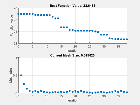
Set options for the patternsearch "nups" algorithm. Set UseVectorized to true, and set options to use the psplotbestf and psplotmeshsize plot functions.
options = optimoptions("patternsearch",...
    UseVectorized=true,Algorithm="nups",...
    MaxFunctionEvaluations=maxf,PlotFcn={"psplotbestf" "psplotmeshsize"});
Call the solver and display the improvement in the sum of squares and the simulation time.
rng(1)
tic
[fittedparamspsn,fvalpsn] = patternsearch(fitobjective,params,[],[],[],[],lb,ub,[],options);
patternsearch stopped because it exceeded options.MaxFunctionEvaluations.
paralleltimepsn = toc
paralleltimepsn =
494.9803
disp([ssq,fvalpsn])
26.9975 22.6433
patternsearch "classic" Algorithm
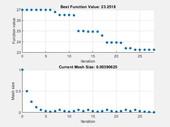
Set options for the patternsearch "classic" algorithm. Set UseVectorized to true, and set options to use the psplotbestf and psplotmeshsize plot functions. To use vectorization with the "classic" algorithm, you must also set the UseCompletePoll option to true.
options = optimoptions("patternsearch",...
    UseVectorized=true,UseCompletePoll=true, ...
    Algorithm="classic",...
    MaxFunctionEvaluations=maxf,PlotFcn={"psplotbestf" "psplotmeshsize"});
tic
[fittedparamspsc,fvalpsc] = patternsearch(fitobjective,params,[],[],[],[],lb,ub,[],options);
patternsearch stopped because it exceeded options.MaxFunctionEvaluations.

paralleltimepsc = toc
paralleltimepsc =
234.5333
disp([ssq,fvalpsc])
26.9975 23.2518
Genetic Algorithm
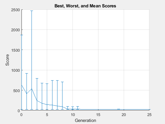
Set options for the genetic algorithm. Set the population size for ga to twice the number of parameters being optimized. Pass the starting point params as the initial population, so that this relatively good point is part of the initial population. To have ga evaluate approximately maxf individuals, set the maximum number of generations to maxf/population size. Set UseVectorized to true.
rng(1)
PopSize = 2*numel(params);
options = optimoptions("ga",PopulationSize=PopSize,...
    UseVectorized=true,InitialPopulationMatrix=params,...
    MaxGenerations=round(maxf/PopSize),PlotFcn="gaplotrange");
tic
[fittedparamsga,fvalga] = ga(fitobjective,numel(params),[],[],[],[],lb,ub,[],options);
ga stopped because it exceeded options.MaxGenerations.
paralleltimega = toc
paralleltimega =
180.8691
disp([ssq,fvalga])
26.9975 24.8405
Surrogate Optimization
Set options for surrogate optimization. Set the BatchSize option to twice the number of parameters being optimized. Set the maximum number of function evaluations to the largest multiple of the batch size that does not exceed maxf. Set UseVectorized to true.
rng(1)
BatchSize = 2*numel(params);
myn = floor(maxf/BatchSize)*BatchSize; % Multiple of BatchSize
options = optimoptions("surrogateopt",BatchUpdateInterval=BatchSize,...
    UseVectorized=true,InitialPoints=params,...
    MaxFunctionEvaluations=myn,PlotFcn="optimplotfvalconstr");
tic
[fittedparamssurr,fvalsurr] = surrogateopt(fitobjective,lb,ub,[],[],[],[],[],options);
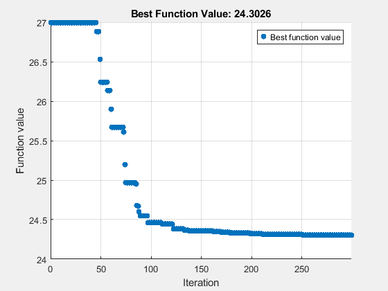
surrogateopt stopped because it exceeded the function evaluation limit set by
'options.MaxFunctionEvaluations'.
paralleltimesur = toc
paralleltimesur =
215.4364
disp([ssq,fvalsurr])
26.9975 24.3026
Particle Swarm Optimization
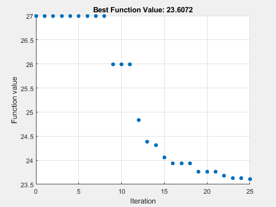
Set options for particle swarm optimization. Set the swarm size to twice the number of parameters being optimized. Set the maximum number of iterations to maxf/swarm size. Set UseVectorized to true.
rng(1)
options = optimoptions("particleswarm",SwarmSize=PopSize,...
    MaxIterations=round(maxf/PopSize),InitialPoints=params,...
    UseVectorized=true,PlotFcn="pswplotbestf");
tic
[fittedparamspsw,fvalpsw] = particleswarm(fitobjective,numel(params),lb,ub,options)
Optimization ended: number of iterations exceeded OPTIONS.MaxIterations.
fittedparamspsw = 1×6

    10.4450    19.8899    9.8416    9.4086    2.6612    27.8898
fvalpsw =
23.6072
paralleltimepsw = toc
paralleltimepsw =
204.0141
disp([ssq,fvalpsw])
26.9975 23.6072
Compare to Nonparallel Computation
For comparison, run the patternsearch "classic" algorithm in serial by setting the UseVectorized option to false.
options = optimoptions("patternsearch",...
    UseVectorized=false,UseCompletePoll=true, ...
    Algorithm="classic",...
    MaxFunctionEvaluations=maxf,PlotFcn={"psplotbestf" "psplotmeshsize"});
tic
[fittedparamspscs,fvalpscs] = patternsearch(fitobjective,params,[],[],[],[],lb,ub,[],options);
patternsearch stopped because it exceeded options.MaxFunctionEvaluations.
serialltimepscs = toc
serialltimepscs =
2.1359e+03
disp([ssq,fvalpscs])
26.9975 23.2518
The nonvectorized (serial) optimization takes much longer than the vectorized (parallel) optimization, and reaches the same solution as the parallel patternsearch "classic" algorithm.
Summarize Results
Collect the results on timing and the best function value for each solver.
table(["NUPS";"PSClassic";"ga";"surr";"particleswarm";"PSClassicSerial"],...
[paralleltimepsn;paralleltimepsc;paralleltimega;paralleltimesur;paralleltimepsw;serialltimepscs], ...
[fvalpsn;fvalpsc;fvalga;fvalsurr;fvalpsw;fvalpscs],...
VariableNames=["Algorithm" "Time" "FVal"])
ans=6×3 table
               "NUPS"      494.9803    22.6433
          "PSClassic"      234.5333    23.2518
                 "ga"      180.8691    24.8405
               "surr"      215.4364    24.3026
      "particleswarm"      204.0141    23.6072
    "PSClassicSerial"    2.1359e+03    23.2518
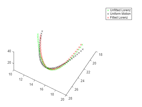
The patternsearch "nups" algorithm has the lowest objective function value. Plot the resulting trajectories for that algorithm.
figure(h)
hold on
in = setparams(in,model,fittedparamspsn);
out = sim(in);
yout = out.yout;
plot3(yout{1}.Values.Data,yout{2}.Values.Data,yout{3}.Values.Data,"rx");
legend("Unfitted Lorenz","Uniform Motion","Fitted Lorenz")
hold off
Conclusion
Using vectorized function calls with parsim can speed the optimization of a Simulink model. All the solvers in this example use the same objective function, which calls a Simulink model to evaluate the objective. The differences in parallel speed are minor, because the simulation takes most of the time, and all the solvers use approximately the same number of function evaluations.
In practice, you might want to use the patternsearch "nups" algorithm first on a problem because, for this example, it reaches the best objective function value. However, different algorithms work better on different problems, so patternsearch "nups" might not be best for your problem.
Helper Functions
This code creates the fitlorenzfn helper function.
function f = fitlorenzfn(x,xdata)
% Lorenz function
theta = x(1:2);
R = x(3);
V = x(4);
t0 = x(5);
delta = x(6:8);
f = zeros(length(xdata),3);
f(:,3) = R*sin(theta(1))*sin(V*(xdata - t0)) + delta(3);
f(:,1) = R*cos(V*(xdata - t0))*cos(theta(2)) ...
    - R*sin(V*(xdata - t0))*cos(theta(1))*sin(theta(2)) + delta(1);
f(:,2) = R*sin(V*(xdata - t0))*cos(theta(1))*cos(theta(2)) ...
    - R*cos(V*(xdata - t0))*sin(theta(2)) + delta(2);
end
This code creates the objfun helper function.
function f = objfun(in,params,YDATA,model)
% Serial one point evaluation of objective
in = setparams(in,model,params);
out = sim(in);
yout = out.yout;
vals = [yout{1}.Values.Data,yout{2}.Values.Data,yout{3}.Values.Data];
f = sum((YDATA - vals).^2,2);
f = sum(f) - (f(1) + f(end))/2;
end
This code creates the setparams helper function.
function pp = setparams(in,model,params)
% parameters [X0,Y0,Z0,Sigma,Beta,Rho]
pp = in.setVariable("X0",params(1),"Workspace",model);
pp = pp.setVariable("Y0",params(2),"Workspace",model);
pp = pp.setVariable("Z0",params(3),"Workspace",model);
pp = pp.setVariable("Sigma",params(4),"Workspace",model);
pp = pp.setVariable("Beta",params(5),"Workspace",model);
pp = pp.setVariable("Rho",params(6),"Workspace",model);
end
This code creates the closeModel helper function.
function closeModel(model)
% To close the model, you must first disable fast restart.
set_param(model,FastRestart="off");
close_system(model)
end
See Also
parsim (Simulink) | ga | particleswarm | patternsearch | surrogateopt