Multi-Object Tracking with DeepSORT

Since R2023b

This example shows how to integrate appearance features from a re-Identification (Re-ID) Deep Neural Network with a multi-object tracker to improve the performance of camera-based object tracking. The implementation closely follows the Deep Simple Online and Realtime (DeepSORT) multi-object tracking algorithm [1]. This example uses the Sensor Fusion and Tracking Toolbox™ and the Computer Vision Toolbox™.

Introduction

The objectives of multi-object tracking are to estimate the number of objects in a scene, to accurately estimate their position, and to establish and maintain unique identities for all objects. You often achieve this through a tracking-by-detection approach that consists of two consecutive tasks. First, you detect objects in each frame using a detector. Then, you track the objects across frames.

This example builds upon the SORT algorithm, introduced in the Implement Simple Online and Realtime Tracking example. The data association and track management of SORT is efficient and simple to implement, but it is ineffective when tracking objects over occlusions in single-view camera scenes.

The increasingly popular Re-ID networks provide appearance features, sometimes called appearance embeddings, for each object detection. Appearance features are a representation of the visual appearance of an object. They offer an additional measure of the similarity (or distance) between a detection and a track. The integration of appearance information into the data association is a powerful technique to handle tracking over longer occlusions and therefore reduces the number of switches in track identities.

Pretrained Person Re-Identification Network

Download the re-identification pretrained network from the internet. Refer to the Reidentify People Throughout a Video Sequence Using ReID Network (Computer Vision Toolbox) example to learn about this network and how to train it. You use this pretrained network to evaluate appearance feature for each detection.

helperDownloadReIDResNet();

Load the Re-ID network.

load("personReIDResNet_v2.mat","net");

To obtain the appearance feature vector of a detection, you extract the bounding box coordinates and convert them to image frame indices. You can then crop out the bounding box of the detection and use the extractReidentificationFeatures (Computer Vision Toolbox) method of the reidentificationNetwork (Computer Vision Toolbox) object to obtain the appearance features. The associationExampleData2 MAT file contains a detection object and a frame, the following code illustrates the use of the extractReidentificationFeatures method.

load("associationExampleData2.mat","detectionBBox","frame");

% Crop frame to measurement bounding box
croppedPerson = imcrop(frame, detectionBBox);
imshow(croppedPerson);

% Extract appearance features of the cropped pedestrian.
appearanceVect = extractReidentificationFeatures(net,croppedPerson)

appearanceVect = 2048×1 single column vector

    -0.4877
     0.3700
    -0.4302
    -0.0238
     0.6064
     0.4683
     0.0888
     0.4270
    -0.0072
    -0.0950
     0.1214
    -0.0945
    -0.0549
    -0.0742
    -0.3841
      ⋮

Use the supporting function runReIDNet to iterate over a set of detections and perform the steps above.

Assignment Metrics

In this section, you learn about the three types of metrics that the DeepSORT assignment strategy relies on.

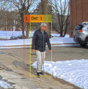
Consider the previous frame and detection. They are depicted in the image below. In the current frame, an object detector returns the detection (Det: 1, in yellow) which should be associated with existing tracks maintained by the multi-object tracker. The tracker hypothesizes that an object with TrackID 1 exist in the current frame, and its estimated bounding box is shown in orange. The track shown on the image is also saved in the associationExampleData2 MAT file.

Each metric type may return values in a different range. Furthermore, some of the metrics measure similarity, where a higher value is preferred, and other metrics are distances, where lower values are preferred. The following paragraphs provide more details on each metric.

load("associationExampleData2.mat","predictedTrack");

Bounding Box Intersection over Union

This is the similarity metric used in SORT as well. It formulates the similarity between a track bounding box and a detection bounding box based on the overlap ratio of the two bounding boxes.

$$\text{similarityIoU}=\frac{\text{Area}\text{of}\text{In}\text{tersection}}{\text{Area}\text{of}\text{Union}}$$

The output, $\text{similarityIoU}$ is a scalar between 0 and 1. A value of 1 indicates that the bounding boxes completely overlap. A value of 0 indicates that there is no intersection. Evaluate the intersection-over-union distance using the distanceIoU function attached to this script.

similarityIoU(predictedTrack, detectionBBox)

ans = 
0.4312

The value computed above shows that the two bounding boxes almost half overlap, which indicates a high similarity, especially in uncrowded scenes.

Mahalanobis Distance

Another common metric is to evaluate the distance between detections and tracks called the Mahalanobis distance, a statistical distance between probability density functions. It accounts for the uncertainty in the current bounding box location estimate and the uncertainty in the measurement. The Mahalanobis distance is nonnegative. A value of 0 indicates no difference between the bounding boxes, in other words, a perfect match. The Mahalanobis distance is technically unbounded. The distance is given by the following equation

$$\text{distanceMahalanobis}={\left(z-\text{Hx}\right)}^T{S}^{-1}\left(z-\text{Hx}\right)$$

$z$ is the bounding box measurement of the detection and $x$ is the track state. $H$ is the Jacobian of the measurement function, which can also be interpreted as the projection from the 8-dimensional state space to the 4-dimensional measurement space in this example. In other words, $\text{Hx}$ is the predicted measurement. $S$ is the innovation covariance matrix with the following definition.

$$S={\text{HPH}}^t+R$$

where $R$ is the measurement noise covariance.

Evaluate the Mahalanobis distance between the predicted track and the detection.

predictedMeasurement = predictedTrack.BoundingBox % Same as Hx

predictedMeasurement = 1×4

    962.4930    353.9284    54.4362    174.6672

innovation = detectionBBox-predictedMeasurement % z - Hx

innovation = 1×4

    16.9370    -0.4384    15.2838    0.7628

predictedCovariance = 24.1729 * eye(4); % Assume the track predicted covariance
R = 25 * eye(4); % Assume the detector accuracy is 5 pixels in each bounding box dimension
S = predictedCovariance + R % Same as HPH' + R

S = 4×4

    49.1729          0          0          0
          0    49.1729          0          0
          0          0    49.1729          0
          0          0          0    49.1729

Finally, calculate the Mahalanobis distance.

distanceManalanobis = innovation / S * innovation'

distanceManalanobis = 
10.5999

Appearance Cosine

This metric evaluates the similarity between a detection and the predicted track in the appearance feature space.

In DeepSORT [1], each track keeps the history of appearance feature vectors from previous detection assignments. For the sake of this example, we saved the track appearance history in the appearanceHistory variable. In this example, appearance vectors are unit vectors with 2048 elements. The following predicted track history has 3 vectors.

load("associationExampleData2.mat","appearanceHistory","detectionAppearance");

The similarity between two appearance vectors is derived directly from their scalar product.

$$d=\frac{⟨{\text{appearance}}_1,{\text{appearance}}_2⟩}{\Vert {\text{appearance}}_1\Vert \Vert {\text{appearance}}_2\Vert }$$

With this formula, you can calculate the similarity between the appearance vector of a detection and the track history as follows. Obviously, the maximum value is 1, when the two vectors are perfectly aligned, and the minimum value is -1, where they are directly opposed to each other.

similarities = (detectionAppearance./vecnorm(detectionAppearance))' *(appearanceHistory./vecnorm(appearanceHistory))

similarities = 1×3 single row vector

    0.8271    0.8846    0.8697

Define the appearance similarity between a track and a detection as the maximum distance across the history of the track appearance vectors, also called a gallery.

appearanceSimilarity = max(similarities)

appearanceSimilarity = single

0.8846

The value computed above is very high and indicates a very good agreement between the appearance features.

In this example you use the three metrics to formulate the overall assignment problem in terms of cost minimization. The tracker you create later in this example uses all three metrics in a matching cascade scheme, which is described in the next section.

Matching Cascade

The original idea behind DeepSORT is to combine the Mahalanobis distance and the appearance feature similarity to assign a set of new detections to the set of current tracks. The combination is done using a weight parameter $\lambda$that has a value between 0 and 1. For the purposes of this cost, we first convert the appearance similarity to a cosine cost, by computing ${\text{Cosine}}_{\text{cost}}=1-\text{appearanceSimilarity}$.

$$\text{Cost}=\lambda {\text{Mahalanobis}}_{\text{Cost}}+\left(1-\lambda \right){\text{Cosine}}_{\text{Cost}}$$

Both Mahalanobis and the appearance cosine cost matrices are subjected to gating thresholds. Thresholding is done by setting cost matrix elements larger than their respective thresholds to Inf. To allow a fair comparison between the unbounded Mahalanobis distance and the cosine cost distance, which is bounded between 0 and 2, both are divided by their gating value.

Due to the growth of the state covariance for unassigned tracks, the Mahalanobis distance tends to favor tracks that have not been updated in the last few frames over tracks with a smaller prediction error. DeepSORT handles this effect by splitting tracks into groups according to the last frame they were assigned. The algorithm assigns tracks that were updated in the previous frame first. Tracks are assigned to the new detections using linear assignment. Any remaining detections are considered for the assignment with the next track group. Once all track groups have been given a chance to get assigned, the remaining unassigned tracks of unassigned age 1, and the remaining unassigned detections are selected for linear assignment based on their IoU cost matrix. The flowchart below describes the matching cascade.

In the next section, you create a video tracker that implements the DeepSORT algorithm.

Build DeepSORT Tracker

After discussing the assignment, the remaining components are the estimation filters, the feature update, and the track initialization and deletion routine. The diagram below gives a summary of all the components involved in tracking-by-detection with DeepSORT.

Use the videoTracker function to create a DeepSORT tracker.

tracker = videoTracker("deepsort");

Specify Video-Related Properties

The tracker works best when configured according to the video frame size and rate. Use the frame variable to define the size. The frame rate is 1 Hz. You can obtain both these values from a video reader configured to your video.

tracker.FrameSize = [size(frame,[1 2])];
tracker.FrameRate = 1;

Matching Cascade

The following properties configure the DeepSORT's matching cascade assignment described in the previous section.

• AppearanceWeight

• MaxMahalanobisDistance

• MinAppearanceSimilarity

• MinIntersectionOverUnion

Set MinIntersectionOverUnion to 0.05 to allow assignment of detections to new tentative tracks with as little as 5% bounding box overlap. In this video, the low frame-rate, the closeness of the camera to the scene, and the small number of people in the scene lead to few and small overlap between consecutive detections. You can set the threshold to a lower value in videos with higher frame-rate or more crowded scenes.

tracker.MinIntersectionOverUnion = 0.05;

Next, set the MaxMahalanobisDistance and MinAppearanceSimilarity properties. The Mahalanobis distance follows a chi-square distribution. Therefore, draw the threshold from the inverse chi-square distribution for a confidence interval of about 95%. For a 4-dimensional measurement space, the value is 9.4877. Manual tuning leads to an appearance threshold of 0.25.

tracker.MaxMahalanobisDistance = 9.4877;
tracker.MinAppearanceSimilarity = 0.25;

In [1], setting the AppearanceWeight $\lambda$to 0 gives better results. In this scene, the combination of the Mahalanobis threshold and the appearance threshold resolves most assignment ambiguities. Therefore, you can choose any value between 0 and 1. For more crowded scenes, consider including some Mahalanobis distance by using non-zero appearance weight as noted in [2]. In this example, a value of 0.5

Track Initialization and Deletion

A new track is confirmed if it has been assigned for 2 consecutive frames. An existing track is deleted if it is missed for more than $T_{\text{Lost}}$ frames. In this example you set $T_{\text{Lost}}=5$. This is long enough to account for all the occlusions in the video which has a low frame-rate (1Hz). For videos with higher frame-rate, you should increase this value accordingly. The following properties allow you to set the confirmation and deletion thresholds.

• NumUpdatesForConfirmation

• NumMissesForDeletion

Set NumUpdatesForConfirmation to [2 2] and NumMissesForDeletion to [$T_{\text{Lost}}$ $T_{\text{Lost}}$] according to the above.

Tlost = 5;
tracker.NumUpdatesForConfirmation = [2 2];
tracker.NumMissesForDeletion = [Tlost Tlost];

Appearance Feature Update

For each assigned track, DeepSORT stores the appearance feature vectors of detections into their assigned tracks. Configure the tracker using the following properties.

• AppearanceUpdate

• MaxNumAppearanceFrames

• AppearanceMomentum

In the original algorithm, DeepSORT stores a gallery of appearance vectors from past frames. Set the AppearanceUpdate property to "Gallery" and the MaxNumAppearanceFrames property to choose the depth of the gallery. You first use a value of 50 frames. Consider increasing this value for high frame-rate videos.

There exist variants of DeepSORT using a different update mechanism [2 ,3]. You can also set AppearanceUpdate to "EMA" to use an exponential moving average update. In this configuration, each track only stores a single appearance vector and updates it with the assigned detection's appearance using the equation:

$${\text{TrackAppearance}}_{k+1}=\alpha {\text{TrackAppearance}}_k+\left(1-\alpha \right)\text{DetectionAppearance}$$

where $\alpha$ is a real value between 0 and 1 called the momentum term.

In this configuration, the MaxNumAppearanceFrames property is not used. Similarly, in the previous gallery configuration, the AppearanceMomentum property is not used.

A second variant consists of combining the exponential moving average with the gallery method. In this method, each track stores a gallery of EMA appearance vector. Set AppearanceUpdate to "EMAGallery" to use this option. Both MaxNumAppearanceFrames and AppearanceMomentum are applicable properties in this configuration.

The gallery method captures long term appearance changes for tracks because it stores previous frames appearances and it does not favor the appearance from the latest frames over older frames. The gallery method is not robust to errors in association for the same reason. Once an erroneous appearance feature is stored in the gallery, it will corrupt the similarity evaluation in later frames (this is due to taking the maximum of similarities across the gallery). The exponential moving average appearance update is more robust to erroneous association since the error will be averaged out, at the expense of not capturing long term appearance change. The exponential moving average gallery offers a compromise between the two methods.

tracker.AppearanceUpdate = "Gallery";
tracker.NumAppearanceFrames = 50;

Evaluate DeepSORT

In this section, you exercise the tracker on the pedestrian tracking video and evaluate its performance using tracking metrics.

Pedestrian Tracking Dataset

Download the pedestrian tracking video file.

helperDownloadPedestrianTrackingVideo();

The PedestrianTrackingYOLODetections MAT file contains detections generated from a YOLO v4 object detector using CSP-DarkNet-53 network and trained on the COCO dataset. See the yolov4ObjectDetector (Computer Vision Toolbox) object for more details. The PedestrianTrackingGroundTruth MAT file contains the ground truth for this video. Refer to the Import Camera-Based Datasets in MOT Challenge Format for Object Tracking example to learn how to import the ground truth and detection data into appropriate Sensor Fusion and Tracking Toolbox formats.

datasetname="PedestrianTracking";
load(datasetname+"GroundTruth.mat","truths");
load(datasetname+"YOLOBboxes.mat","bboxesYOLO");

Run the Tracker with Gallery

Next, exercise the complete tracking workflow on the Pedestrian Tracking video. To use the tracker, call the tracker as if it were a function. The inputs to the tracker are an M-by-4 matrix of bounding box measurements, where each row is a bounding box returned from the detector, and an M-by-N matrix, where each row is an array of appearance features returned from the re-ID network. The tracker returns confirmed tracks as an array of structures.

In the original implementation of DeepSORT, the tracker maintains a gallery of appearance features, which are used for data association. The following code sets up the tracker for this kind of appearance update.

release(tracker); % To allow modifying the following tracker properties.
tracker.AppearanceUpdate = "Gallery";

% Choose the weight between appearance and Mahalanobis
weight =0.5;
tracker.AppearanceWeight = weight;

% Reset the track log
trackLogGallery = struct.empty;

% Create video reader and video player
reader = VideoReader("PedestrianTrackingVideo.avi");
player = vision.DeployableVideoPlayer;

for i=1:reader.NumFrames
    % Advance reader
    frame = readFrame(reader);

    % Run Re-ID Network on detections to get the appearance vectors
    appearances = runReIDNet(net, frame, bboxesYOLO{i});

    % Update the tracker with bounding boxes and appearance vectors
    tracks = tracker(bboxesYOLO{i}, appearances);

    % Visualize the tracks
    if ~isempty(tracks)
        trackColors = getTrackColors(tracks);
        frame = insertObjectAnnotation(frame, 'Rectangle', vertcat(tracks.BoundingBox),...
            vertcat(tracks.TrackID), Color=trackColors, TextBoxOpacity=0.8);
    end
    step(player, frame);

    % Log tracks for evaluation. Delete tracks that are outside the frame
    % for a fair comparison with the truth that does not contain objects
    % outside the frame.
    trackToDelete = areTracksOutOfFrame(tracks);
    tracks = tracks(~trackToDelete); 
    trackLogGallery = [trackLogGallery ; tracks]; %#ok<AGROW>
end

From the results, the person tracked with ID = 3 is occluded multiple times and makes abrupt change of direction. This makes it difficult to track with only motion information by the means of the Mahalanobis distance or bounding box overlap. The use of appearance feature allows to maintain a unique track identifier for this person over this entire sequence and for the rest of the video. This is not achieved with the simpler SORT algorithm or when setting DeepSORT to only use the Mahalanobis distance.

DeepSORT Variations

The literature contains variations of DeepSORT, which are different from each other in the way the appearance features are maintained and used for data association. In the following code, you run the "EMA" and "EMAGallery" variations to see how using them impacts tracking quality.

trackLogEMA = rerunTracker(tracker, "EMA", weight, reader, net, bboxesYOLO);
trackLogEMAGallery = rerunTracker(tracker, "EMAGallery", weight, reader, net, bboxesYOLO);

Tracking Metrics

The CLEAR multi-object tracking metrics provide a standard set of tracking metrics to evaluate the quality of tracking algorithm. These metrics are popular for video-based tracking applications. Use the trackCLEARMetrics object to evaluate the CLEAR metrics for the two SORT runs.

The CLEAR metrics require a similarity method to match track and true object pairs in each frame. In this example, you use the IoU2d similarity method and set the SimilarityThreshold property to 0.01. This means that a track can only be considered a true positive match with a truth object if their bounding boxes overlap by at least 1%. The metric results can vary depending on the choice of this threshold.

tcm = trackCLEARMetrics(SimilarityMethod ="IoU2d", SimilarityThreshold = 0.01);

To evaluate the results on the Pedestrian class only, you only keep ground truth elements with ClassID equal to 1 and filter out other classes.

truths = truths([truths.ClassID]==1);

Use the evaluate object function to obtain the metrics as a table for each one of the appearance update options.

resultsGallery = evaluate(tcm, trackLogGallery, truths);
resultsEMA = evaluate(tcm, trackLogEMA, truths);
resultsEMAGallery = evaluate(tcm, trackLogEMAGallery, truths);
allResults = [table("Gallery",VariableNames = "AppearanceUpdate") , resultsGallery ; ...
    table("EMA",VariableNames = "AppearanceUpdate"), resultsEMA; ...
    table("EMAGallery",VariableNames = "AppearanceUpdate"), resultsEMAGallery];

disp(allResults);

    AppearanceUpdate    MOTA (%)    MOTP (%)    Mostly Tracked (%)    Partially Tracked (%)    Mostly Lost (%)    False Positive    False Negative    Recall (%)    Precision (%)    False Track Rate    ID Switches    Fragmentations
    ________________    ________    ________    __________________    _____________________    _______________    ______________    ______________    __________    _____________    ________________    ___________    ______________

      "Gallery"          89.701      92.057           92.308                 7.6923                   0                 23                39            93.522         96.075            0.13609              0               5       
      "EMA"              90.698      92.151           92.308                 7.6923                   0                 18                38            93.688         96.907            0.10651              0               4       
      "EMAGallery"       90.698      92.151           92.308                 7.6923                   0                 18                38            93.688         96.907            0.10651              0               4       

The CLEAR MOT metrics corroborate the quality of DeepSORT in keeping identities of tracks over time with no ID switch and very little fragmentation. This is the main benefit of using DeepSORT over SORT. Meanwhile, maintaining tracks alive over occlusions results in predicted locations being maintained (coasting) and compared against true position, which leads to increased number of false positives and false negatives when the overlap between the coasted tracks and true bounding boxes is less than the metric threshold. This is reflected in the MOTA score of DeepSORT.

When comparing the different AppearanceUpdate options, the metrics show that in this case the "EMA" and "EMAGallery" outperform the "Gallery" option in terms of overall MOTA and MOTP, reduced number of false positives, false negatives, and fragmentations. Since the "EMA" option is also the most efficient in terms of computations and memory usage, it is recommended to use "EMA" in this case. Videos taken in other settings, especially ones where the scene is very crowded or contains regions with shaded and well-lit areas, may be better served with a different appearance update option. Having all three update mechanisms available as options in the tracker allows you to find the best solution for your use case and setting.

Refer to the trackCLEARMetrics page for additional information about all the CLEAR metrics quantities.

Conclusion

In this example you have learned how to implement the DeepSORT object tracking algorithm. This is an example of attribute fusion by using deep appearance features for the assignment. The appearance attribute is updated using a simple memory buffer. You also have learned how to integrate a Re-Identification Deep Learning network as part of the tracking-by-detection framework to improve the performance of camera-based tracking in the presence of occlusions.

Additionally, this example showed how to configure the tracker to use different methods to maintain the appearance features in the track and compared their results.

Supporting Functions

runReIDNet runs the re-ID network on a set of bounding boxes in a frame and returns a set of feature vectors as a matrix.

function appearances = runReIDNet(net, frame, bboxes)

numBboxes = size(bboxes,1);
appearances = zeros(numBboxes,2048,'like',bboxes);
for j =1:numBboxes

    % Crop frame
    bbox = bboxes(j,:);
    croppedPerson = imcrop(frame,bbox);

    % Extract appearance features of the cropped pedestrian.
    appearances(j,:) = extractReidentificationFeatures(net,croppedPerson);
end
end

areTracksOutOfFrame returns a logical array of tracks whose bounding box is entirely out of the video frame.

function isOutOfFrame = areTracksOutOfFrame(confirmedTracks)
% Get bounding boxes
allboxes = vertcat(confirmedTracks.BoundingBox);
allboxes = max(allboxes, realmin);
alloverlaps = bboxOverlapRatio(allboxes,[1,1,1288,964]);
isOutOfFrame = ~alloverlaps;
end

similarityIoU Calculates the similarity between a track and detection based on the intersection-over-union metric.

function iou = similarityIoU(track, detectorBBox)
trackBBox = [track.BoundingBox];


% left top corner
x1BboxA = trackBBox(:, 1);
y1BboxA = trackBBox(:, 2);
% right bottom corner
x2BboxA = x1BboxA + trackBBox(:, 3);
y2BboxA = y1BboxA + trackBBox(:, 4);

x1BboxB = detectorBBox(:, 1);
y1BboxB = detectorBBox(:, 2);
x2BboxB = x1BboxB + detectorBBox(:, 3);
y2BboxB = y1BboxB + detectorBBox(:, 4);

% area of the bounding box
areaA = trackBBox(:, 3) .* trackBBox(:, 4);
areaB = detectorBBox(:, 3) .* detectorBBox(:, 4);

iou = ones(size(trackBBox,1),size(detectorBBox,1), 'like', trackBBox);

for m = 1:size(trackBBox,1)
    for n = 1:size(detectorBBox,1)
        % compute the corners of the intersect
        x1 = max(x1BboxA(m), x1BboxB(n));
        y1 = max(y1BboxA(m), y1BboxB(n));
        x2 = min(x2BboxA(m), x2BboxB(n));
        y2 = min(y2BboxA(m), y2BboxB(n));

        % skip if there is no intersection
        w = x2 - x1;
        if w <= 0
            continue;
        end

        h = y2 - y1;
        if h <= 0
            continue;
        end

        intersectAB = w * h;
        iou(m,n) = intersectAB/(areaA(m)+areaB(n)-intersectAB);
    end
end
end

rerunTracker rerun the tracker with a new appearance update method and weight and return a track log for evaluation

function tracklog = rerunTracker(tracker, update, weight, reader, reIDNet, bboxes)
release(tracker); % To allow modifying the following tracker properties.
tracker.AppearanceUpdate = update;
tracker.AppearanceMomentum = 0.7;

% Choose cost appearance weight
tracker.AppearanceWeight = weight;

% Reset the track log
tracklog = struct.empty;

% Create video reader and video player
player = vision.DeployableVideoPlayer;

% Reset the reader
reader.CurrentTime = 0;

for i=1:reader.NumFrames
    % Advance reader
    frame = readFrame(reader);

    % Run Re-ID Network on detections
    appearances = runReIDNet(reIDNet, frame, bboxes{i});

    % Run the tracker on bounding boxes and appearance vectors
    tracks = tracker(bboxes{i}, appearances);

    % Display the tracks
    if ~isempty(tracks)
        trackColors = getTrackColors(tracks);
        frame = insertObjectAnnotation(frame, 'Rectangle', vertcat(tracks.BoundingBox),vertcat(tracks.TrackID),'Color',trackColors, 'TextBoxOpacity',0.8);
    end
    step(player, frame);

    % Delete tracks out of frame and log the remaining tracks for evaluation
    trackToDelete = areTracksOutOfFrame(tracks);
    tracks = tracks(~trackToDelete); 
    tracklog = [tracklog ; tracks]; %#ok<AGROW>
end
end

getTrackColors Returns track colors based on track IDs.

function colors = getTrackColors(tracks)
colors = zeros(numel(tracks), 3);
coloroptions = 255*lines(7);
for i=1:numel(tracks)
    colors(i,:) = coloroptions(mod(tracks(i).TrackID, 7)+1,:);
end
end

Reference

[1] Wojke, Nicolai, Alex Bewley, and Dietrich Paulus. "Simple online and realtime tracking with a deep association metric." In 2017 IEEE international conference on image processing (ICIP), pp. 3645-3649.

[2] Du, Yunhao, Zhicheng Zhao, Yang Song, Yanyun Zhao, Fei Su, Tao Gong, and Hongying Meng. "Strongsort: Make deepsort great again." IEEE Transactions on Multimedia (2023).

[3] Du, Yunhao, Junfeng Wan, Yanyun Zhao, Binyu Zhang, Zhihang Tong, and Junhao Dong. "Giaotracker: A comprehensive framework for mcmot with global information and optimizing strategies in visdrone 2021." In Proceedings of the IEEE/CVF International conference on computer vision, pp. 2809-2819. 2021.