Implement Simple Online and Realtime Tracking
This example shows how to implement the Simple Online and Realtime (SORT) object tracking algorithm [1] using the Sensor Fusion and Tracking Toolbox™ and the Computer Vision Toolbox™. The example also shows how to evaluate SORT with the CLEAR MOT metrics.
Download Pedestrian Tracking Video
Download the pedestrian tracking video file.
datasetname = "PedestrianTracking";
videoURL = "https://ssd.mathworks.com/supportfiles/vision/data/PedestrianTrackingVideo.avi";
if ~exist("PedestrianTrackingVideo.avi","file")
    disp("Downloading Pedestrian Tracking Video (35 MB)")
    websave("PedestrianTrackingVideo.avi",videoURL);
end
Downloading Pedestrian Tracking Video (35 MB)
Open the video in a video reader.
reader = VideoReader(datasetname+"Video.avi");Refer to the Import Camera-Based Datasets in MOT Challenge Format for Object Tracking example to learn how to import the ground truth data into appropriate Sensor Fusion and Tracking Toolbox formats. You use the same pedestrian tracking dataset in this example.
In this example, you implement a SORT tracker and use it to track pedestrians using two detectors: The peopleDetectorACF and the YOLOv4 detector. Having two detector types allows you to compare the tracking quality and observe the detector impact on the tracking results.
Define SORT Video Tracker
To implement a SORT tracker, use the videoTracker function and "sort" as the algorithm name. The function creates a task-oriented tracker specifically designed for tracking objects in a video frame. The tracker input is bounding boxes obtained from a video detector.
tracker = videoTracker("sort");To enable the tracker to work correctly, you must specify the frame size and rate based on your video. You can get these values directly from the video reader.
tracker.FrameSize = [reader.Width reader.Height];
tracker.FrameRate = reader.FrameRate;
Like any other multi-object tracking algorithms, setting a threshold for the association of detections to tracks is beneficial. The SORT algorithm uses the intersection-over-union (IoU) metric to evaluate similarity between detector bounding boxes and track bounding boxes. An IoU value of 1 indicates that the two bounding boxes match perfectly in both position and dimensions and a value of 0 indicates no overlap.
Depending on the video frame rate, the speed at which objects are moving, and the detector accuracy, you will need to reduce the threshold to make sure that the tracker is able to associate detections to tracks. For the video used in this example, a minimum similarity value of 0.03 gives good results due to the low density of pedestrian and the low frame rate. Therefore, set the MinIntersectionOverUnion property of the tracker to the IoUmin of your choice using the slide below.
IoUmin = 0.03;
tracker.MinIntersectionOverUnion = IoUmin;
0.03;
tracker.MinIntersectionOverUnion = IoUmin;Define Track Maintenance
Objects can leave the video frame or become occluded for brief or long periods. You need to define the maximum number of frames without assigned detections, , before deleting a track. The tracker parameter can be tuned for each application and a value of 3 shows good results for this video. Additionally, SORT requires an object to be detected in two consecutive frames before confirming a track. You set the NumUpdatesForConfirmation property of the tracker accordingly.
tracker.NumUpdatesForConfirmation = [2 2]; TLost =3; % Number of consecutive missed frames to delete a track tracker.NumMissesForDeletion = [TLost TLost];
Run SORT with ACF Detections
Run SORT on the video and detections. Filter out ACF detections with a score lower than 15 to improve the tracking performance. You can tune the score threshold for specific scenarios. Log the tracks at each time step for offline evaluation. You exclude tracks that are outside the frame as these do not exist in the truth data and would present as false positives if included when calculating the CLEAR metrics.
% Create the ACF people detector
detector = peopleDetectorACF;
detectionScoreThreshold = 15;

% Initialize track log
acfSORTTrackLog = struct.empty;

% Reset the reader and the tracker
reader.CurrentTime = 0;
reset(tracker);

for i=1:reader.NumFrames
    % Advance reader
    frame = readFrame(reader);

    % Detect objects in the frame using the detector
    [boundingBoxes,scores] = detect(detector,frame);

    % Uncomment the line below to show detection
    % frame = insertObjectAnnotation(frame,'Rectangle',boundingBoxes,scores,TextBoxOpacity=0.2);

    % Update tracker with bounding boxes that pass the score threshold
    highScoreBBoxes = boundingBoxes(scores >= detectionScoreThreshold,:);
    tracks = tracker(highScoreBBoxes);

    % Visualize the tracks
    if ~isempty(tracks)
        trackPositions = vertcat(tracks.BoundingBox);
        trackIDs = [tracks.TrackID];
        trackColors = getTrackColors(tracks);
        frame = insertObjectAnnotation(frame,"Rectangle",trackPositions,"T"+trackIDs, ...
            Color=trackColors,TextBoxOpacity=0.8);
    end

    imshow(frame);
    drawnow limitrate

    % Log tracks for evaluation
    trackToDelete = areTracksOutOfFrame(tracks);
    tracks = tracks(~trackToDelete);
    acfSORTTrackLog = [acfSORTTrackLog; tracks]; %#ok<AGROW>
end
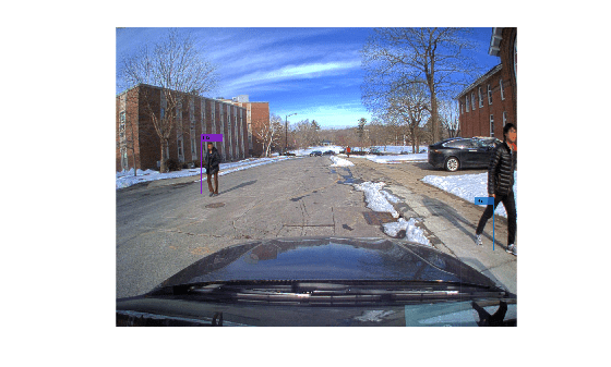
By the end of the video, a pedestrian is tracked with a trackID of 45. The sequence contains exactly 16 distinct pedestrians. Apparently, the tracker has confirmed new tracks for the same true object several times as well as possibly confirmed false positive tracks.
SORT can struggle to initiate for tracking fast moving objects because it initializes a tentative track in the first frame with zero velocity and the detection of the same object in the next frame may not overlap with the prediction. This challenge is further accentuated in videos with low frame rate like the video in this example. For instance, track 3 is not confirmed until visible for multiple frames.
Notice that pedestrians who leave the field of view of the camera or are occluded by another person for a few frames are lost by the tracker. This result is a combination of using the constant velocity model to predict the position of the track and using the IoU association cost, which cannot associate a predicted track to a new detection if the positions are too far.
The quality of the detections also has noticeable impacts on tracking results. For example, the ACF detections of the tree at the end of the street are associated to track 3. You can reduce the number of false measurements like that by increasing the score threshold to more than 15. However, a high threshold will reduce the number of detections reported to the tracker, and for high enough threshold, it may lead to filtering good detections from the tracker.
In the next section, you evaluate SORT with the YOLOv4 detections.
Run SORT with YOLOv4 Detections
In this section you run SORT with the detections obtained from the YOLOv4 detector. For the YOLOv4 detector, the detection quality is sufficiently good such that you can skip the optional step of filtering low quality detections before sending them to the tracker. However, since we are only interested in tracking pedestrians, we still need to filter the bounding boxes based on their class. In this section, use detections that were recorded from the YOLO detector to avoid the need to download the YOLOv4 support package.
% Create the YOLO detector
load("PedestrainYOLOBboxes.mat","bboxesYOLO");

% Initialize track log
yoloSORTTrackLog = struct.empty;

% Reset the reader and the tracker
reader.CurrentTime = 0;
reset(tracker);

for i=1:reader.NumFrames
    % Advance reader
    frame = readFrame(reader);

    % Update tracker with recorded YOLO detections
    tracks = tracker(bboxesYOLO{i});

    % Visualize the tracks
    if ~isempty(tracks)
        trackIDs = [tracks.TrackID];
        trackColors = getTrackColors(tracks);
        frame = insertObjectAnnotation(frame, 'Rectangle',vertcat(tracks.BoundingBox),"T"+trackIDs, ...
            Color=trackColors, TextBoxOpacity=0.8);
    end
    imshow(frame);
    drawnow limitrate

    % Log tracks for evaluation
    trackToDelete = areTracksOutOfFrame(tracks);
    tracks = tracks(~trackToDelete);
    yoloSORTTrackLog = [yoloSORTTrackLog; tracks]; %#ok<AGROW>
end
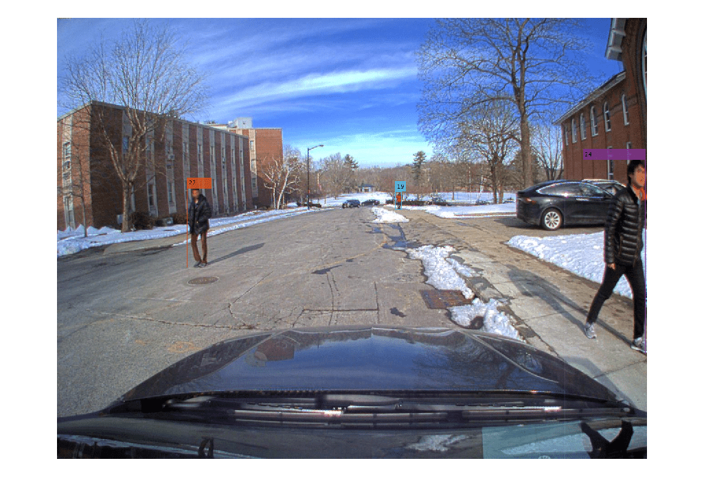
The YOLOv4-SORT combination created a total of 22 tracks on the video, indicating that fewer track fragmentations occurred as compared to the ACF detections. By inspecting the video, some ID switches are still noticeable.
More recent tracking algorithms, such as DeepSORT, modify the association cost to include appearance features in addition to IoU. These algorithms show great improvements in accuracy and are able to keep tracks over longer occlusions thanks to re-identification networks.
Evaluate SORT with the CLEAR MOT Metrics
The CLEAR multi-object tracking metrics provide a standard set of tracking metrics to evaluate the quality of tracking algorithm [2]. These metrics are popular for video-based tracking applications. Use the trackCLEARMetrics object to evaluate the CLEAR metrics for the two SORT runs.
The CLEAR metrics require a similarity method to match track and true object pairs in each frame. In this example, you use the IoU2d similarity method and set the SimilarityThreshold property to 0.1. This means that a track can only be considered a true positive match with a truth object if their bounding boxes overlap by at least 10%. The metric results can vary depending on the choice of this threshold.
threshold =0.1; tcm = trackCLEARMetrics(SimilarityMethod="IoU2d", SimilarityThreshold=threshold);
The PedestrianTrackingGroundTruth MAT file contains the log of truth objects formatted as an array of structures. Each structure contains the following fields: TruthID, Time, and BoundingBox. After loading the ground truth, call the evaluate object function to obtain the metrics as a table.
load("PedestrianTrackingGroundTruth.mat","truths");
acfSORTresults = evaluate(tcm, acfSORTTrackLog, truths);
yoloSORTresults = evaluate(tcm, yoloSORTTrackLog, truths);
Concatenate the two tables and add a column with the name of each tracker and object detector.
allResults = [table("ACF+SORT",VariableNames = "Tracker") , acfSORTresults ; ...
    table("YOLOv4+SORT",VariableNames = "Tracker"), yoloSORTresults];

disp(allResults);
       Tracker       MOTA (%)    MOTP (%)    Mostly Tracked (%)    Partially Tracked (%)    Mostly Lost (%)    False Positive    False Negative    Recall (%)    Precision (%)    False Track Rate    ID Switches    Fragmentations
    _____________    ________    ________    __________________    _____________________    _______________    ______________    ______________    __________    _____________    ________________    ___________    ______________

    "ACF+SORT"        68.981      67.375           64.286                 28.571                7.1429               21               174            73.148         95.758             0.12426             6               8
    "YOLOv4+SORT"     83.951      90.708           78.571                 14.286                7.1429               12                92            85.802         97.887            0.071006             0               9
The two main summary metrics are Multi-Object Tracking Accuracy (MOTA) and Multi-Object Tracking Precision (MOTP). MOTA is a good indicator of the data association quality while MOTP indicates the similarity of each track bounding boxes with their matched true bounding boxes. The metrics confirm that the YOLOv4 and SORT combination tracks better than the ACF and SORT combination. It scores roughly 15 percent higher for both MOTA and MOTP, which shows the importance of having a good detector that can accurately detect and report bounding boxes of desired objects.
ID switches and fragmentations are two other metrics that provide good insights on a tracker's ability to track each pedestrian with a unique track ID. Fragmentations can occur when a true object is obstructed and the tracker cannot maintain the track continuously over several frames. ID switches can occur when true objects trajectories are crossing and their assigned track IDs switch afterwards.
Refer to the trackCLEARMetrics page for additional information about all the CLEAR metrics quantities and their significance.
Conclusion
In this example you learned how to use the SORT videoTracker. Also, you evaluated this tracking algorithm on a pedestrian tracking video. You discovered that the overall tracking performance depends strongly on the quality of the detections. You can reuse this example with your own video and detections. Furthermore, you can use the Import Camera-Based Datasets in MOT Challenge Format for Object Tracking example to import videos and detections from the MOT Challenge.
Reference
[1] Bewley, Alex, Zongyuan Ge, Lionel Ott, Fabio Ramos, and Ben Upcroft. "Simple online and realtime tracking." In 2016 IEEE international conference on image processing (ICIP), pp. 3464-3468. IEEE, 2016.
[2] Bernardin, Keni, and Rainer Stiefelhagen. "Evaluating multiple object tracking performance: the clear mot metrics." EURASIP Journal on Image and Video Processing 2008 (2008): 1-10.
Supporting Functions
getTrackColors Return colors associated with the tracks based on track ID.
function colors = getTrackColors(tracks)
colors = zeros(numel(tracks), 3);
coloroptions = 255*lines(7);
for i=1:numel(tracks)
    colors(i,:) = coloroptions(mod(tracks(i).TrackID, 7)+1,:);
end
end
areTracksOutOfFrame returns a logical array of tracks whose bounding box is entirely out of the video frame.
function isOutOfFrame = areTracksOutOfFrame(confirmedTracks)
% Get bounding boxes
allboxes = vertcat(confirmedTracks.BoundingBox);
allboxes = max(allboxes, realmin);
alloverlaps = bboxOverlapRatio(allboxes,[1,1,1288,964]);
isOutOfFrame = ~alloverlaps;
end