partitionDetections
Partition detections based on distance
Syntax
Description
A partition of a set of detections is defined as a division of these detections
into nonempty mutually exclusive detection cells. Using multiple distance thresholds, you can
use the function to separate detections into different detection cells and get all the
possible partitions using either distance-partitioning or
density-based spatial clustering of applications with noise (DBSCAN).
Additionally, you can choose the distance metric as Mahalanobis distance or Euclidean distance
by specifying the 'Distance' Name-Value pair argument.
Distance Partitioning
Distance partitioning is the default partitioning algorithm of
partitionDetections. In distance partitioning, a detection cluster
comprises of detections whose distance to at least one other detection in the cluster is
less than the distance threshold. In other words, two detections belong to the same
detection cluster if their distance is less than the distance threshold. To use
distance-partitioning, you can specify the 'Algorithm' Name-Value
argument as 'Distance-Partitioning' or simply do not specify the
'Algorithm' argument.
partitions = partitionDetections(detections)detections using the
distance-partitioning algorithm. By default, the function uses the distance partitioning
algorithm and considers all real value Mahalanobis distance thresholds between 0.5 and
6.25 and returns a maximum of 100 partitions.
partitions = partitionDetections(detections,tLower,tUpper)tLower and tUpper.
partitions = partitionDetections(detections,tLower,tUpper,'MaxNumPartitions',maxNumber)maxNumber.
partitions = partitionDetections(detections,allThresholds)
[
additionally returns an index vector partitions,indexDP] = partitionDetections(detections,allThresholds)indexDP representing the
correspondence between all thresholds and the resulting partitions.
DBSCAN Partitioning
To use the DBSCAN partitioning, specify the 'Algorithm' argument as
'DBSCAN'.
partitions = partitionDetections(detections,'Algorithm','DBSCAN')
partitions = partitionDetections(detections,epsilon,minNumPoints,'Algorithm','DBSCAN')epsilon and the minimum number of
points per cluster minNumPoints of the DBSCAN algorithm.
[
additionally returns an index vector partitions,indexDB] = partitionDetections(detections,epsilon,minNumPoints,'Algorithm','DBSCAN')indexDB representing the
correspondence between the threshold values epsilon and the resulting
partitions.
Specify Distance Metric
Using the 'Distance' Name-Value argument, you can specify the
distance metric used in the partitioning.
___ = partitionDetections(___,'Distance',
additionally specifies the distance metric as distance)'Mahalanobis' or
'Euclidean'. Use this syntax with any of the input or output
arguments in previous syntaxes.
Examples
Generate 2-D detections using objectDetection.
rng(2018); % For reproducible results
detections = cell(10,1);
for i = 1:numel(detections)
    id = randi([1 5]);
    detections{i} = objectDetection(0,[id;id] + 0.1*randn(2,1));
    detections{i}.MeasurementNoise = 0.01*eye(2);
end
Extract and display generated position measurements.
d = [detections{:}];
measurements = [d.Measurement];

figure()
plot(measurements(1,:),measurements(2,:),'x','MarkerSize',10,'MarkerEdgeColor','b')
title('Measurements')
xlabel('x')
ylabel('y')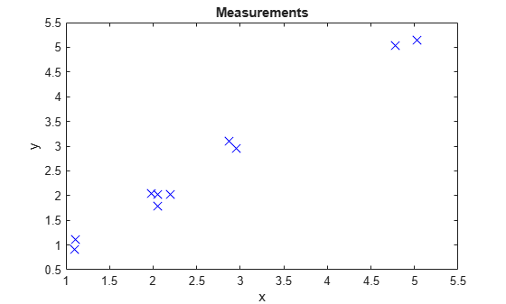
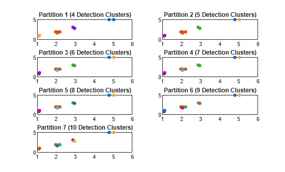
Generate partitions from the detections using distance partitioning and count the number of partitions.
partitions = partitionDetections(detections);
numPartitions = size(partitions,2);
Visualize the partitions. Each color represents a detection cluster.
figure()
for i = 1:numPartitions
    numCells = max(partitions(:,i));
    subplot(4,ceil(numPartitions/4),i);
    for k = 1:numCells
        ids = partitions(:,i) == k;
        plot(measurements(1,ids),measurements(2,ids),'.','MarkerSize',15);
        hold on;
    end
    title(['Partition ',num2str(i),' (',num2str(k),' Detection Clusters)']);
end
Generate 2-D detections using objectDetection.
rng(2018); % For reproducible results
detections = cell(10,1);
for i = 1:numel(detections)
    id = randi([1 5]);
    detections{i} = objectDetection(0,[id;id] + 0.1*randn(2,1));
    detections{i}.MeasurementNoise = 0.01*eye(2);
end
Extract and display generated position measurements.
d = [detections{:}];
measurements = [d.Measurement];

figure()
plot(measurements(1,:),measurements(2,:),'x','MarkerSize',10,'MarkerEdgeColor','b')
title('Measurements')
xlabel('x')
ylabel('y')
Generate partitions from the detections using DBSCAN and count the number of partitions.
[partitions,index] = partitionDetections(detections,[1.6;2],2,'Algorithm','DBSCAN');
numPartitions = size(partitions,2);
Visualize the partitions. Each color represents a detection cluster.
figure()
for i = 1:numPartitions
    numCells = max(partitions(:,i));
    subplot(2,ceil(numPartitions/2),i);
    for k = 1:numCells
        ids = partitions(:,i) == k;
        plot(measurements(1,ids),measurements(2,ids),'.','MarkerSize',15);
        hold on;
    end
    title(['Partition ',num2str(i),' (',num2str(k),' Detection Clusters)']);
end

From the index values, the first partition corresponds to an epsilon value of 2 and the second partition corresponds to an epsilon value of 1.6.
index
index = 1×2 uint32 row vector

   2   1
Input Arguments
Output Arguments
References
[1] Granstrom, Karl, Christian Lundquist, and Omut Orguner. “Extended Target Tracking Using a Gaussian-Mixture PHD Filter.” IEEE Transactions on Aerospace and Electronic Systems 48, no. 4 (October 2012): 3268–86. https://doi.org/10.1109/TAES.2012.6324703.
[2] Ester, Martin, Hans-Peter Kriegel, Jörg Sander, and Xiaowei Xu. “A Density-Based Algorithm for Discovering Clusters in Large Spatial Databases with Noise.” In Proceedings of the Second International Conference on Knowledge Discovery and Data Mining, 226–31. KDD’96. Portland, Oregon: AAAI Press, 1996.
Extended Capabilities
Version History
Introduced in R2019a