Graphical Representation of Trees
Introduction
You can use the function
treeviewer to display a
graphical representation of a tree, allowing you to examine interactively the prices
and rates on the nodes of the tree until maturity. To get started with this process,
first load the data file deriv.mat included in this
toolbox.
load deriv.mat
Note
treeviewer price tree diagrams follow the convention that
increasing prices appear on the upper branch of a tree and, consequently,
decreasing prices appear on the lower branch. Conversely, for interest rate
displays, decreasing interest rates appear on the upper
branch (prices are rising) and increasing interest rates on
the lower branch (prices are falling).
For information on the use of treeviewer to observe interest
rate movement, see Observing Interest Rates.
For information on using treeviewer to observe the
movement of prices, see Observing Instrument Prices.
Observing Interest Rates
If you provide the name of an interest rate tree to the treeviewer function, it displays
a graphical view of the path of interest rates. For example, here is the treeviewer representation of all
the rates along both the up and down branches of HJMTree.
treeviewer(HJMTree)
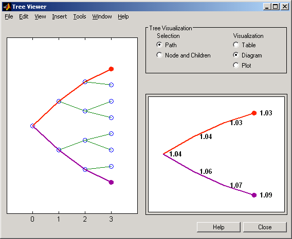
The example in Examining Trees used
bushpath to find the path of
forward rates along an HJM tree by taking the first branch up and then two branches
down the rate tree.
FRates = bushpath(HJMTree.FwdTree, [1 2 2])
FRates =

    1.0356
    1.0364
    1.0526
    1.0674
With the treeviewer function you can
display the identical information by clicking along the same sequence of nodes, as
shown next.
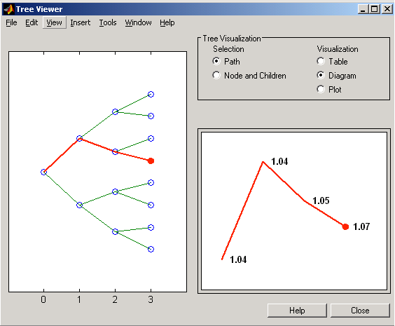
Next is a treeviewer representation of
interest rates along several branches of BDTTree.
treeviewer(BDTTree)

Note
When using treeviewer with recombining trees,
such as BDT, BK, and HW, you must click each node in succession from the
beginning to the end. Because these trees can recombine, treeviewer is unable to
complete the path automatically.
The example in Examining Trees used
treepath to find the path of
interest rates taking the first branch up and then two branches down the rate
tree.
FRates = treepath(BDTTree.FwdTree, [1 2 2])
FRates =

    1.1000
    1.0979
    1.1377
    1.1606
You can display the identical information by clicking along the same sequence of nodes, as shown next.

Observing Instrument Prices
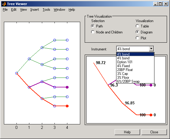
To use treeviewer to display a tree of
instrument prices, provide the name of an instrument set along with the name of a
price tree in your call to treeviewer, for example:
load deriv.mat
[Price, PriceTree] = hjmprice(HJMTree, HJMInstSet);
treeviewer(PriceTree, HJMInstSet)
With treeviewer you select
each instrument individually in the instrument portfolio
for display.
You can use an analogous process to view instrument prices based on the BDT
interest rate tree included in deriv.mat.
load deriv.mat
[BDTPrice, BDTPriceTree] = bdtprice(BDTTree, BDTInstSet);
treeviewer(BDTPriceTree, BDTInstSet)

Valuation Date Prices
You can use treeviewer
instrument-by-instrument to observe instrument prices through time. For the
first 4% bond in the HJM instrument portfolio, treeviewer indicates a
valuation date price of 98.72, the same value obtained by accessing the
PriceTree structure directly.

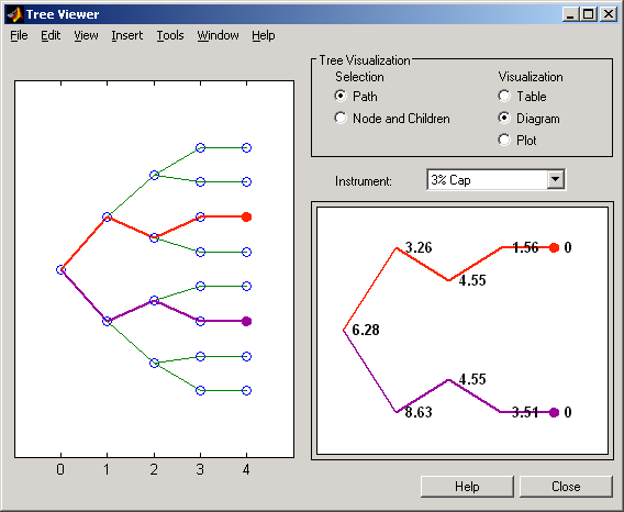
As a further example, look at the sixth instrument in the price vector, the 3%
cap. At the valuation date, its value obtained directly from the structure is
6.2831. Use treeviewer on this
instrument to confirm this price.
Additional Observation Times
The second node represents the first-rate observation time, tObs =
1. This node displays two states, one representing the branch
going up and the other one representing the branch going down.
Examine the prices of the node corresponding to the up branch.
PriceTree.PBush{2}(:,:,1)ans =
100.1563
99.7309
0.1007
100.1563
100.3782
3.2594
0.1007
3.5597
As before, you can use treeviewer, this time to
examine the price for the 4% bond on the up branch. treeviewer displays a price
of 100.2 for the first node of the up branch, as expected.

Now examine the corresponding down branch.
PriceTree.PBush{2}(:,:,2)ans =
96.3041
94.1986
0
96.3041
100.3671
8.6342
0
-0.3923
Use treeviewer once again, now
to observe the price of the 4% bond on the down branch. The displayed price of
96.3 conforms to the price obtained from direct access of the
PriceTree structure. You may continue this process as far
along the price tree as you want.

See Also
instbond | instcap | instcf | instfixed | instfloat | instfloor | instoptbnd | instoptembnd | instoptfloat | instoptemfloat | instrangefloat | instswap | instswaption | intenvset | bondbyzero | cfbyzero | fixedbyzero | floatbyzero | intenvprice | intenvsens | swapbyzero | floatmargin | floatdiscmargin | hjmtimespec | hjmtree | hjmvolspec | bondbyhjm | capbyhjm | cfbyhjm | fixedbyhjm | floatbyhjm | floorbyhjm | hjmprice | hjmsens | mmktbyhjm | oasbyhjm | optbndbyhjm | optfloatbyhjm | optembndbyhjm | optemfloatbyhjm | rangefloatbyhjm | swapbyhjm | swaptionbyhjm | bdttimespec | bdttree | bdtvolspec | bdtprice | bdtsens | bondbybdt | capbybdt | cfbybdt | fixedbybdt | floatbybdt | floorbybdt | mmktbybdt | oasbybdt | optbndbybdt | optfloatbybdt | optembndbybdt | optemfloatbybdt | rangefloatbybdt | swapbybdt | swaptionbybdt | hwtimespec | hwtree | hwvolspec | bondbyhw | capbyhw | cfbyhw | fixedbyhw | floatbyhw | floorbyhw | hwcalbycap | hwcalbyfloor | hwprice | hwsens | oasbyhw | optbndbyhw | optfloatbyhw | optembndbyhw | optemfloatbyhw | rangefloatbyhw | swapbyhw | swaptionbyhw | bktimespec | bktree | bkvolspec | bkprice | bksens | bondbybk | capbybk | cfbybk | fixedbybk | floatbybk | floorbybk | oasbybk | optbndbybk | optfloatbybk | optembndbybk | optemfloatbybk | rangefloatbybk | swapbybk | swaptionbybk | capbyblk | floorbyblk | swaptionbyblk
Topics
- Overview of Interest-Rate Tree Models
- Pricing Using Interest-Rate Term Structure
- Pricing Using Interest-Rate Tree Models
- Understanding Interest-Rate Tree Models
- Understanding Interest-Rate Term Structure
- Supported Interest-Rate Instrument Functions
- Supported Equity Derivative Functions
- Supported Energy Derivative Functions