Plot Efficient Frontier of Financial Portfolios

This example analyzes three portfolios with given rates of return for six time periods by executing MATLAB^® functions using Spreadsheet Link™. In actual practice, these functions can analyze many portfolios over many time periods, limited only by the amount of computer memory available.

For details about the efficient frontier of financial portfolios, see Analyzing Portfolios (Financial Toolbox). To learn about portfolio optimization theory, see Portfolio Optimization Theory (Financial Toolbox).

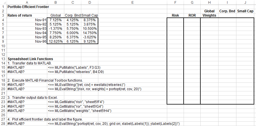
The example organizes and displays the input and output data in a Microsoft^® Excel^® worksheet. Spreadsheet Link functions copy data to a MATLAB matrix, perform calculations using Financial Toolbox™ functions, and return data to the worksheet.

Open the ExliSamp.xls file and select the Sheet5 worksheet. For help finding the ExliSamp.xls file, see Installation.

This worksheet contains rates of return for three different portfolios: Global, Corporate Bond, and Small Cap.

Note

This example requires Financial Toolbox, Statistics and Machine Learning Toolbox™, and Optimization Toolbox™.

1. Execute the Spreadsheet Link function that transfers the plot labels for the x-axis and y-axis to the MATLAB workspace by double-clicking the cell A15 and pressing Enter.

2. Copy the portfolio return data to the MATLAB workspace by executing the function in the cell A16.

3. Generate efficient frontier data for 20 points along the frontier by executing the Financial Toolbox functions in A19 and A20.

4. Copy the output data to the Excel worksheet by executing the Spreadsheet Link functions in A23, A24, and A25.

   The output data contains the highest rate of return ROR for a given risk. The output data also contains the weighted investment in each portfolio Weights that achieves that rate of return.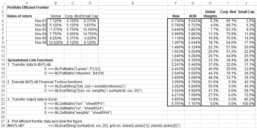

   

5. Plot the efficient frontier for the same portfolio data by executing the Financial Toolbox functions in cell A28.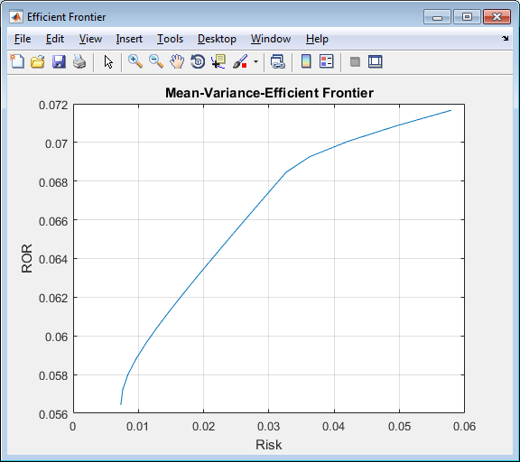

   

   The light blue line shows the efficient frontier. Observe the change in slope above a 6.8% return because the Corporate Bond portfolio no longer contributes to the efficient frontier.

To generate different efficient frontier data, close the figure and change the data in cells B4:D9. Then, execute all the Spreadsheet Link functions again. The worksheet updates with new frontier data and MATLAB generates a new efficient frontier plot.