Compare One-Sided and Two-Sided Hodrick-Prescott Filter Results

Smooth the quarterly U.S. Gross Domestic Product (GDP) series by applying the Hodrick-Prescott filter. Compare the smoothed trend components returned from the one-sided and two-sided methods. Use interactive controls to experiment with parameter settings interactively.

The standard, two-sided Hodrick-Prescott filter [1] computes a centered difference to estimate a second derivative at time $\mathit{t}$, $\mathit{t}=1,...,\mathit{T}$, using both past and future values of the input series. Although past and future values, relative to $\mathit{t}$, are available for input historical series, in real time, future values are not known leading to anomalous end effects. As a result, the filtered data can be unsuitable for forecasting [2].

The one-sided Hodrick-Prescott filter [2] uses, at each time $\mathit{t}$, only current and previous values of the input series; it does not revise outputs when new data is available.

Load the U.S. GDP data set Data_GDP.mat, which contains quarterly measurements from 1947 through 2005.

load Data_GDP

The data set contains a timetable DataTimeTable, among other variables, containing the series.

Plot the raw series. Indicate periods of recession in the plot by drawing vertical bands.

figure
plot(DataTimeTable.Time,DataTimeTable.GDP)
recessionplot
ylabel("Billions of Dollars")
title("Gross Domestic Product")

The GDP tends to increase with time also displaying a cycle with the upward trend.

Decompose the series into trend and cyclical components using the standard, two-sided Hodrick-Prescott filter. Because the series is quarterly, use the default smoothing parameter value. Return the third output to plot the data series and the smoothed trend.

figure
[TTbl2S,CTbl2S,h] = hpfilter(DataTimeTable);
legend(h,AutoUpdate="off",Location="best")
recessionplot

TTbl2S and CTbl2S are timetables containing variables for the additive smoothed trend and cyclical components, respectively, of the GDP.

The trend appears quite smooth with mild oscillations.

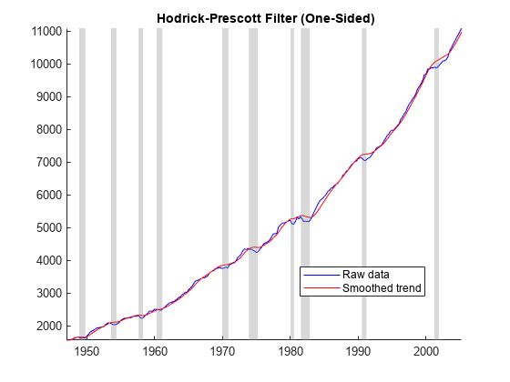
Decompose the series again using the one-sided Hodrick-Prescott filter by setting the FilterType name-value argument.

figure
[TTbl1S,CTbl1S,h] = hpfilter(DataTimeTable,FilterType="one-sided");
legend(h,AutoUpdate="off",Location="best")
recessionplot

The trend of the one-sided filter appears to level sharply close to recessions, as compared to the smooth trend of the two-sided filter.

Plot the cyclical components computed from both filter methods on the same plot.

figure
hold on
plot(CTbl2S.Time,CTbl2S.GDP,"r")
plot(CTbl1S.Time,CTbl1S.GDP,"r:",LineWidth=2)
recessionplot
hold off
ylabel("Cyclical Component")
title("Gross Domestic Product")
legend(["Two-Sided HP Cycle","One-Sided HP Cycle"])

The cyclical components appear to be distinct calibrations of forecasting models.

Interactive Controls enable you to experiment with the smoothing parameter and the filter type interactively.

Choose the filter type by using the drop-down list and adjust the smoothing parameter by using the numeric slider.

ft = "one-sided"; % FilterType
lambda = 1600; % Smoothing

figure
[TTbl1S,CTbl1S,h] = hpfilter(DataTimeTable,FilterType=ft,Smoothing=lambda);
legend(h,AutoUpdate="off",Location="best")
recessionplot

References

[1] Hodrick, Robert J., and Edward C. Prescott. "Postwar U.S. Business Cycles: An Empirical Investigation." Journal of Money, Credit and Banking 29, no. 1 (February 1997): 1–16. https://doi.org/10.2307/2953682.

[2] Stock, James H., and Mark W. Watson. "Forecasting Inflation." Journal of Monetary Economics 44, no. 2 (October 1999): 293–335. https://doi.org/10.1016/S0304-3932(99)00027-6.

[3] U.S. Federal Reserve Economic Data (FRED), Federal Reserve Bank of St. Louis, https://fred.stlouisfed.org/.